MATHHX B
\(\newcommand{\footnotename}{footnote}\)
\(\def \LWRfootnote {1}\)
\(\newcommand {\footnote }[2][\LWRfootnote ]{{}^{\mathrm {#1}}}\)
\(\newcommand {\footnotemark }[1][\LWRfootnote ]{{}^{\mathrm {#1}}}\)
\(\let \LWRorighspace \hspace \)
\(\renewcommand {\hspace }{\ifstar \LWRorighspace \LWRorighspace }\)
\(\newcommand {\TextOrMath }[2]{#2}\)
\(\newcommand {\mathnormal }[1]{{#1}}\)
\(\newcommand \ensuremath [1]{#1}\)
\(\newcommand {\LWRframebox }[2][]{\fbox {#2}} \newcommand {\framebox }[1][]{\LWRframebox } \)
\(\newcommand {\setlength }[2]{}\)
\(\newcommand {\addtolength }[2]{}\)
\(\newcommand {\setcounter }[2]{}\)
\(\newcommand {\addtocounter }[2]{}\)
\(\newcommand {\arabic }[1]{}\)
\(\newcommand {\number }[1]{}\)
\(\newcommand {\noalign }[1]{\text {#1}\notag \\}\)
\(\newcommand {\cline }[1]{}\)
\(\newcommand {\directlua }[1]{\text {(directlua)}}\)
\(\newcommand {\luatexdirectlua }[1]{\text {(directlua)}}\)
\(\newcommand {\protect }{}\)
\(\def \LWRabsorbnumber #1 {}\)
\(\def \LWRabsorbquotenumber "#1 {}\)
\(\newcommand {\LWRabsorboption }[1][]{}\)
\(\newcommand {\LWRabsorbtwooptions }[1][]{\LWRabsorboption }\)
\(\def \mathchar {\ifnextchar "\LWRabsorbquotenumber \LWRabsorbnumber }\)
\(\def \mathcode #1={\mathchar }\)
\(\let \delcode \mathcode \)
\(\let \delimiter \mathchar \)
\(\def \oe {\unicode {x0153}}\)
\(\def \OE {\unicode {x0152}}\)
\(\def \ae {\unicode {x00E6}}\)
\(\def \AE {\unicode {x00C6}}\)
\(\def \aa {\unicode {x00E5}}\)
\(\def \AA {\unicode {x00C5}}\)
\(\def \o {\unicode {x00F8}}\)
\(\def \O {\unicode {x00D8}}\)
\(\def \l {\unicode {x0142}}\)
\(\def \L {\unicode {x0141}}\)
\(\def \ss {\unicode {x00DF}}\)
\(\def \SS {\unicode {x1E9E}}\)
\(\def \dag {\unicode {x2020}}\)
\(\def \ddag {\unicode {x2021}}\)
\(\def \P {\unicode {x00B6}}\)
\(\def \copyright {\unicode {x00A9}}\)
\(\def \pounds {\unicode {x00A3}}\)
\(\let \LWRref \ref \)
\(\renewcommand {\ref }{\ifstar \LWRref \LWRref }\)
\( \newcommand {\multicolumn }[3]{#3}\)
\(\require {textcomp}\)
\(\require {colortbl}\)
\(\let \LWRorigcolumncolor \columncolor \)
\(\renewcommand {\columncolor }[2][named]{\LWRorigcolumncolor [#1]{#2}\LWRabsorbtwooptions }\)
\(\let \LWRorigrowcolor \rowcolor \)
\(\renewcommand {\rowcolor }[2][named]{\LWRorigrowcolor [#1]{#2}\LWRabsorbtwooptions }\)
\(\let \LWRorigcellcolor \cellcolor \)
\(\renewcommand {\cellcolor }[2][named]{\LWRorigcellcolor [#1]{#2}\LWRabsorbtwooptions }\)
\(\newcommand {\tothe }[1]{^{#1}}\)
\(\newcommand {\raiseto }[2]{{#2}^{#1}}\)
\(\newcommand {\LWRsiunitxEND }{}\)
\(\def \LWRsiunitxang #1;#2;#3;#4\LWRsiunitxEND {\ifblank {#1}{}{\num {#1}\degree }\ifblank {#2}{}{\num {#2}^{\unicode {x2032}}}\ifblank {#3}{}{\num {#3}^{\unicode {x2033}}}}\)
\(\newcommand {\ang }[2][]{\LWRsiunitxang #2;;;\LWRsiunitxEND }\)
\(\def \LWRsiunitxdistribunit {}\)
\(\newcommand {\LWRsiunitxENDTWO }{}\)
\(\def \LWRsiunitxprintdecimalsubtwo #1,#2,#3\LWRsiunitxENDTWO {\ifblank {#1}{0}{\mathrm {#1}}\ifblank {#2}{}{{\LWRsiunitxdecimal }\mathrm {#2}}}\)
\(\def \LWRsiunitxprintdecimalsub #1.#2.#3\LWRsiunitxEND {\LWRsiunitxprintdecimalsubtwo #1,,\LWRsiunitxENDTWO \ifblank {#2}{}{{\LWRsiunitxdecimal }\LWRsiunitxprintdecimalsubtwo
#2,,\LWRsiunitxENDTWO }}\)
\(\newcommand {\LWRsiunitxprintdecimal }[1]{\LWRsiunitxprintdecimalsub #1...\LWRsiunitxEND }\)
\(\def \LWRsiunitxnumplus #1+#2+#3\LWRsiunitxEND {\ifblank {#2}{\LWRsiunitxprintdecimal {#1}}{\ifblank {#1}{\LWRsiunitxprintdecimal {#2}}{\LWRsiunitxprintdecimal {#1}\unicode
{x02B}\LWRsiunitxprintdecimal {#2}}}\LWRsiunitxdistribunit }\)
\(\def \LWRsiunitxnumminus #1-#2-#3\LWRsiunitxEND {\ifblank {#2}{\LWRsiunitxnumplus #1+++\LWRsiunitxEND }{\ifblank {#1}{}{\LWRsiunitxprintdecimal {#1}}\unicode {x02212}\LWRsiunitxprintdecimal
{#2}\LWRsiunitxdistribunit }}\)
\(\def \LWRsiunitxnumpmmacro #1\pm #2\pm #3\LWRsiunitxEND {\ifblank {#2}{\LWRsiunitxnumminus #1---\LWRsiunitxEND }{\LWRsiunitxprintdecimal {#1}\unicode {x0B1}\LWRsiunitxprintdecimal
{#2}\LWRsiunitxdistribunit }}\)
\(\def \LWRsiunitxnumpm #1+-#2+-#3\LWRsiunitxEND {\ifblank {#2}{\LWRsiunitxnumpmmacro #1\pm \pm \pm \LWRsiunitxEND }{\LWRsiunitxprintdecimal {#1}\unicode {x0B1}\LWRsiunitxprintdecimal
{#2}\LWRsiunitxdistribunit }}\)
\(\newcommand {\LWRsiunitxnumscientific }[2]{\ifblank {#1}{}{\ifstrequal {#1}{-}{-}{\LWRsiunitxprintdecimal {#1}\times }}10^{\LWRsiunitxprintdecimal {#2}}\LWRsiunitxdistribunit }\)
\(\def \LWRsiunitxnumD #1D#2D#3\LWRsiunitxEND {\ifblank {#2}{\LWRsiunitxnumpm #1+-+-\LWRsiunitxEND }{\mathrm {\LWRsiunitxnumscientific {#1}{#2}}}}\)
\(\def \LWRsiunitxnumd #1d#2d#3\LWRsiunitxEND {\ifblank {#2}{\LWRsiunitxnumD #1DDD\LWRsiunitxEND }{\mathrm {\LWRsiunitxnumscientific {#1}{#2}}}}\)
\(\def \LWRsiunitxnumE #1E#2E#3\LWRsiunitxEND {\ifblank {#2}{\LWRsiunitxnumd #1ddd\LWRsiunitxEND }{\mathrm {\LWRsiunitxnumscientific {#1}{#2}}}}\)
\(\def \LWRsiunitxnume #1e#2e#3\LWRsiunitxEND {\ifblank {#2}{\LWRsiunitxnumE #1EEE\LWRsiunitxEND }{\mathrm {\LWRsiunitxnumscientific {#1}{#2}}}}\)
\(\def \LWRsiunitxnumx #1x#2x#3x#4\LWRsiunitxEND {\ifblank {#2}{\LWRsiunitxnume #1eee\LWRsiunitxEND }{\ifblank {#3}{\LWRsiunitxnume #1eee\LWRsiunitxEND \times \LWRsiunitxnume
#2eee\LWRsiunitxEND }{\LWRsiunitxnume #1eee\LWRsiunitxEND \times \LWRsiunitxnume #2eee\LWRsiunitxEND \times \LWRsiunitxnume #3eee\LWRsiunitxEND }}}\)
\(\newcommand {\num }[2][]{\LWRsiunitxnumx #2xxxxx\LWRsiunitxEND }\)
\(\newcommand {\si }[2][]{\mathrm {\gsubstitute {#2}{~}{\,}}}\)
\(\def \LWRsiunitxSIopt #1[#2]#3{\def \LWRsiunitxdistribunit {\,\si {#3}}{#2}\num {#1}\def \LWRsiunitxdistribunit {}}\)
\(\newcommand {\LWRsiunitxSI }[2]{\def \LWRsiunitxdistribunit {\,\si {#2}}\num {#1}\def \LWRsiunitxdistribunit {}}\)
\(\newcommand {\SI }[2][]{\ifnextchar [{\LWRsiunitxSIopt {#2}}{\LWRsiunitxSI {#2}}}\)
\(\newcommand {\numlist }[2][]{\text {#2}}\)
\(\newcommand {\numrange }[3][]{\num {#2}\ \LWRsiunitxrangephrase \ \num {#3}}\)
\(\newcommand {\SIlist }[3][]{\text {#2}\,\si {#3}}\)
\(\newcommand {\SIrange }[4][]{\num {#2}\,#4\ \LWRsiunitxrangephrase \ \num {#3}\,#4}\)
\(\newcommand {\tablenum }[2][]{\mathrm {#2}}\)
\(\newcommand {\ampere }{\mathrm {A}}\)
\(\newcommand {\candela }{\mathrm {cd}}\)
\(\newcommand {\kelvin }{\mathrm {K}}\)
\(\newcommand {\kilogram }{\mathrm {kg}}\)
\(\newcommand {\metre }{\mathrm {m}}\)
\(\newcommand {\mole }{\mathrm {mol}}\)
\(\newcommand {\second }{\mathrm {s}}\)
\(\newcommand {\becquerel }{\mathrm {Bq}}\)
\(\newcommand {\degreeCelsius }{\unicode {x2103}}\)
\(\newcommand {\coulomb }{\mathrm {C}}\)
\(\newcommand {\farad }{\mathrm {F}}\)
\(\newcommand {\gray }{\mathrm {Gy}}\)
\(\newcommand {\hertz }{\mathrm {Hz}}\)
\(\newcommand {\henry }{\mathrm {H}}\)
\(\newcommand {\joule }{\mathrm {J}}\)
\(\newcommand {\katal }{\mathrm {kat}}\)
\(\newcommand {\lumen }{\mathrm {lm}}\)
\(\newcommand {\lux }{\mathrm {lx}}\)
\(\newcommand {\newton }{\mathrm {N}}\)
\(\newcommand {\ohm }{\mathrm {\Omega }}\)
\(\newcommand {\pascal }{\mathrm {Pa}}\)
\(\newcommand {\radian }{\mathrm {rad}}\)
\(\newcommand {\siemens }{\mathrm {S}}\)
\(\newcommand {\sievert }{\mathrm {Sv}}\)
\(\newcommand {\steradian }{\mathrm {sr}}\)
\(\newcommand {\tesla }{\mathrm {T}}\)
\(\newcommand {\volt }{\mathrm {V}}\)
\(\newcommand {\watt }{\mathrm {W}}\)
\(\newcommand {\weber }{\mathrm {Wb}}\)
\(\newcommand {\day }{\mathrm {d}}\)
\(\newcommand {\degree }{\mathrm {^\circ }}\)
\(\newcommand {\hectare }{\mathrm {ha}}\)
\(\newcommand {\hour }{\mathrm {h}}\)
\(\newcommand {\litre }{\mathrm {l}}\)
\(\newcommand {\liter }{\mathrm {L}}\)
\(\newcommand {\arcminute }{^\prime }\)
\(\newcommand {\minute }{\mathrm {min}}\)
\(\newcommand {\arcsecond }{^{\prime \prime }}\)
\(\newcommand {\tonne }{\mathrm {t}}\)
\(\newcommand {\astronomicalunit }{au}\)
\(\newcommand {\atomicmassunit }{u}\)
\(\newcommand {\bohr }{\mathit {a}_0}\)
\(\newcommand {\clight }{\mathit {c}_0}\)
\(\newcommand {\dalton }{\mathrm {D}_\mathrm {a}}\)
\(\newcommand {\electronmass }{\mathit {m}_{\mathrm {e}}}\)
\(\newcommand {\electronvolt }{\mathrm {eV}}\)
\(\newcommand {\elementarycharge }{\mathit {e}}\)
\(\newcommand {\hartree }{\mathit {E}_{\mathrm {h}}}\)
\(\newcommand {\planckbar }{\mathit {\unicode {x210F}}}\)
\(\newcommand {\angstrom }{\mathrm {\unicode {x212B}}}\)
\(\let \LWRorigbar \bar \)
\(\newcommand {\barn }{\mathrm {b}}\)
\(\newcommand {\bel }{\mathrm {B}}\)
\(\newcommand {\decibel }{\mathrm {dB}}\)
\(\newcommand {\knot }{\mathrm {kn}}\)
\(\newcommand {\mmHg }{\mathrm {mmHg}}\)
\(\newcommand {\nauticalmile }{\mathrm {M}}\)
\(\newcommand {\neper }{\mathrm {Np}}\)
\(\newcommand {\yocto }{\mathrm {y}}\)
\(\newcommand {\zepto }{\mathrm {z}}\)
\(\newcommand {\atto }{\mathrm {a}}\)
\(\newcommand {\femto }{\mathrm {f}}\)
\(\newcommand {\pico }{\mathrm {p}}\)
\(\newcommand {\nano }{\mathrm {n}}\)
\(\newcommand {\micro }{\mathrm {\unicode {x00B5}}}\)
\(\newcommand {\milli }{\mathrm {m}}\)
\(\newcommand {\centi }{\mathrm {c}}\)
\(\newcommand {\deci }{\mathrm {d}}\)
\(\newcommand {\deca }{\mathrm {da}}\)
\(\newcommand {\hecto }{\mathrm {h}}\)
\(\newcommand {\kilo }{\mathrm {k}}\)
\(\newcommand {\mega }{\mathrm {M}}\)
\(\newcommand {\giga }{\mathrm {G}}\)
\(\newcommand {\tera }{\mathrm {T}}\)
\(\newcommand {\peta }{\mathrm {P}}\)
\(\newcommand {\exa }{\mathrm {E}}\)
\(\newcommand {\zetta }{\mathrm {Z}}\)
\(\newcommand {\yotta }{\mathrm {Y}}\)
\(\newcommand {\percent }{\mathrm {\%}}\)
\(\newcommand {\meter }{\mathrm {m}}\)
\(\newcommand {\metre }{\mathrm {m}}\)
\(\newcommand {\gram }{\mathrm {g}}\)
\(\newcommand {\kg }{\kilo \gram }\)
\(\newcommand {\of }[1]{_{\mathrm {#1}}}\)
\(\newcommand {\squared }{^2}\)
\(\newcommand {\square }[1]{\mathrm {#1}^2}\)
\(\newcommand {\cubed }{^3}\)
\(\newcommand {\cubic }[1]{\mathrm {#1}^3}\)
\(\newcommand {\per }{\,\mathrm {/}}\)
\(\newcommand {\celsius }{\unicode {x2103}}\)
\(\newcommand {\fg }{\femto \gram }\)
\(\newcommand {\pg }{\pico \gram }\)
\(\newcommand {\ng }{\nano \gram }\)
\(\newcommand {\ug }{\micro \gram }\)
\(\newcommand {\mg }{\milli \gram }\)
\(\newcommand {\g }{\gram }\)
\(\newcommand {\kg }{\kilo \gram }\)
\(\newcommand {\amu }{\mathrm {u}}\)
\(\newcommand {\nm }{\nano \metre }\)
\(\newcommand {\um }{\micro \metre }\)
\(\newcommand {\mm }{\milli \metre }\)
\(\newcommand {\cm }{\centi \metre }\)
\(\newcommand {\dm }{\deci \metre }\)
\(\newcommand {\m }{\metre }\)
\(\newcommand {\km }{\kilo \metre }\)
\(\newcommand {\as }{\atto \second }\)
\(\newcommand {\fs }{\femto \second }\)
\(\newcommand {\ps }{\pico \second }\)
\(\newcommand {\ns }{\nano \second }\)
\(\newcommand {\us }{\micro \second }\)
\(\newcommand {\ms }{\milli \second }\)
\(\newcommand {\s }{\second }\)
\(\newcommand {\fmol }{\femto \mol }\)
\(\newcommand {\pmol }{\pico \mol }\)
\(\newcommand {\nmol }{\nano \mol }\)
\(\newcommand {\umol }{\micro \mol }\)
\(\newcommand {\mmol }{\milli \mol }\)
\(\newcommand {\mol }{\mol }\)
\(\newcommand {\kmol }{\kilo \mol }\)
\(\newcommand {\pA }{\pico \ampere }\)
\(\newcommand {\nA }{\nano \ampere }\)
\(\newcommand {\uA }{\micro \ampere }\)
\(\newcommand {\mA }{\milli \ampere }\)
\(\newcommand {\A }{\ampere }\)
\(\newcommand {\kA }{\kilo \ampere }\)
\(\newcommand {\ul }{\micro \litre }\)
\(\newcommand {\ml }{\milli \litre }\)
\(\newcommand {\l }{\litre }\)
\(\newcommand {\hl }{\hecto \litre }\)
\(\newcommand {\uL }{\micro \liter }\)
\(\newcommand {\mL }{\milli \liter }\)
\(\newcommand {\L }{\liter }\)
\(\newcommand {\hL }{\hecto \liter }\)
\(\newcommand {\mHz }{\milli \hertz }\)
\(\newcommand {\Hz }{\hertz }\)
\(\newcommand {\kHz }{\kilo \hertz }\)
\(\newcommand {\MHz }{\mega \hertz }\)
\(\newcommand {\GHz }{\giga \hertz }\)
\(\newcommand {\THz }{\tera \hertz }\)
\(\newcommand {\mN }{\milli \newton }\)
\(\newcommand {\N }{\newton }\)
\(\newcommand {\kN }{\kilo \newton }\)
\(\newcommand {\MN }{\mega \newton }\)
\(\newcommand {\Pa }{\pascal }\)
\(\newcommand {\kPa }{\kilo \pascal }\)
\(\newcommand {\MPa }{\mega \pascal }\)
\(\newcommand {\GPa }{\giga \pascal }\)
\(\newcommand {\mohm }{\milli \ohm }\)
\(\newcommand {\kohm }{\kilo \ohm }\)
\(\newcommand {\Mohm }{\mega \ohm }\)
\(\newcommand {\pV }{\pico \volt }\)
\(\newcommand {\nV }{\nano \volt }\)
\(\newcommand {\uV }{\micro \volt }\)
\(\newcommand {\mV }{\milli \volt }\)
\(\newcommand {\V }{\volt }\)
\(\newcommand {\kV }{\kilo \volt }\)
\(\newcommand {\W }{\watt }\)
\(\newcommand {\uW }{\micro \watt }\)
\(\newcommand {\mW }{\milli \watt }\)
\(\newcommand {\kW }{\kilo \watt }\)
\(\newcommand {\MW }{\mega \watt }\)
\(\newcommand {\GW }{\giga \watt }\)
\(\newcommand {\J }{\joule }\)
\(\newcommand {\uJ }{\micro \joule }\)
\(\newcommand {\mJ }{\milli \joule }\)
\(\newcommand {\kJ }{\kilo \joule }\)
\(\newcommand {\eV }{\electronvolt }\)
\(\newcommand {\meV }{\milli \electronvolt }\)
\(\newcommand {\keV }{\kilo \electronvolt }\)
\(\newcommand {\MeV }{\mega \electronvolt }\)
\(\newcommand {\GeV }{\giga \electronvolt }\)
\(\newcommand {\TeV }{\tera \electronvolt }\)
\(\newcommand {\kWh }{\kilo \watt \hour }\)
\(\newcommand {\F }{\farad }\)
\(\newcommand {\fF }{\femto \farad }\)
\(\newcommand {\pF }{\pico \farad }\)
\(\newcommand {\K }{\mathrm {K}}\)
\(\newcommand {\dB }{\mathrm {dB}}\)
\(\newcommand {\kibi }{\mathrm {Ki}}\)
\(\newcommand {\mebi }{\mathrm {Mi}}\)
\(\newcommand {\gibi }{\mathrm {Gi}}\)
\(\newcommand {\tebi }{\mathrm {Ti}}\)
\(\newcommand {\pebi }{\mathrm {Pi}}\)
\(\newcommand {\exbi }{\mathrm {Ei}}\)
\(\newcommand {\zebi }{\mathrm {Zi}}\)
\(\newcommand {\yobi }{\mathrm {Yi}}\)
\(\let \unit \si \)
\(\let \qty \SI \)
\(\let \qtylist \SIlist \)
\(\let \qtyrange \SIrange \)
\(\let \numproduct \num \)
\(\let \qtyproduct \SI \)
\(\let \complexnum \num \)
\(\newcommand {\complexqty }[3][]{(\complexnum {#2})\si {#3}}\)
\(\newcommand {\mleft }{\left }\)
\(\newcommand {\mright }{\right }\)
\(\newcommand {\mleftright }{}\)
\(\newcommand {\mleftrightrestore }{}\)
\(\require {gensymb}\)
\(\newcommand {\intertext }[1]{\text {#1}\notag \\}\)
\(\let \Hat \hat \)
\(\let \Check \check \)
\(\let \Tilde \tilde \)
\(\let \Acute \acute \)
\(\let \Grave \grave \)
\(\let \Dot \dot \)
\(\let \Ddot \ddot \)
\(\let \Breve \breve \)
\(\let \Bar \bar \)
\(\let \Vec \vec \)
\(\require {cancel}\)
\(\newcommand {\mathred }[1]{\textcolor [rgb]{1, 0, 0}{#1}}\)
\(\newcommand {\mathgreen }[1]{\textcolor [rgb]{0,0.5,0}{#1}}\)
\(\newcommand {\mathblue }[1]{\textcolor [rgb]{0,0,1}{#1}}\)
\(\newcommand {\mathorange }[1]{\textcolor [rgb]{1,0.5,0}{#1}}\)
\(\newcommand {\mathmagenta }[1]{\textcolor [cmyk]{0, 1, 1, 0.33}{#1}}\)
\( \newcommand \ccancel [2][red]{\renewcommand \CancelColor {\color {#1}}\cancel {#2}} \)
\(\newcommand {\Dom }{\operatorname {Dom}}\)
\(\newcommand {\Ran }{\operatorname {Ran}}\)
\(\newcommand {\Dm }{\operatorname {Dm}}\)
\(\newcommand {\Vm }{\operatorname {Vm}}\)
\(\newcommand {\Var }{\operatorname {Var}}\)
\(\newcommand {\SD }{\operatorname {SD}}\)
\(\newcommand {\ExV }{\operatorname {E}}\)
\(\newcommand {\opointtext }{\textcolor {blue}{\circ }}\)
\(\newcommand {\cpointtext }{\textcolor {blue}{\bullet }}\)
\(\newcommand {\vectwo }[2]{\begin {pmatrix} #1 \\ #2 \end {pmatrix}}\)
\(\newcommand {\tcbset }[1]{}\)
\(\newcommand {\tcbsetforeverylayer }[1]{}\)
\(\newcommand {\tcbox }[2][]{\boxed {\text {#2}}}\)
\(\newcommand {\tcboxfit }[2][]{\boxed {#2}}\)
\(\newcommand {\tcblower }{}\)
\(\newcommand {\tcbline }{}\)
\(\newcommand {\tcbtitle }{}\)
\(\newcommand {\tcbsubtitle [2][]{\mathrm {#2}}}\)
\(\newcommand {\tcboxmath }[2][]{\boxed {#2}}\)
\(\newcommand {\tcbhighmath }[2][]{\boxed {#2}}\)
\(\newcommand {\toprule }[1][]{\hline }\)
\(\let \midrule \toprule \)
\(\let \bottomrule \toprule \)
\(\def \LWRbooktabscmidruleparen (#1)#2{}\)
\(\newcommand {\LWRbooktabscmidrulenoparen }[1]{}\)
\(\newcommand {\cmidrule }[1][]{\ifnextchar (\LWRbooktabscmidruleparen \LWRbooktabscmidrulenoparen }\)
\(\newcommand {\morecmidrules }{}\)
\(\newcommand {\specialrule }[3]{\hline }\)
\(\newcommand {\addlinespace }[1][]{}\)
\(\def \LWRsiunitxrangephrase {\TextOrMath { }{\ }\protect \mbox {to (numerical range)}\TextOrMath { }{\ }}\)
\(\def \LWRsiunitxdecimal {.}\)
2.4 Nulpunkter og fortegnsundersøgelse
Vi husker, at vi indfører nye begreber i matematik ved at opskrive definitioner. I dette afsnit skal vi først kigge på begrebet nulpunkt, og derfor starter vi med at opskrive definitionen af et nulpunkt.
-
Definition 2.4.1
Lad \(f\) være en funktion.
Et nulpunkt for \(f\) er en \(x\)-værdi, som har en funktionsværdi på nul.
Så selvom det hedder et nulpunkt, er det altså en \(x\)-værdi og ikke et punkt.
-
Eksempel 2.4.1
Lad \(f(x)=2x-6\).
Vi vil undersøge, om \(x=3\) er et nulpunkt for \(f\), så vi regner \(f(3)\):
\[ f(3) = 2\cdot 3-6 =0 \]
Da \(f(3)=0\), er \(x=3\) et nulpunkt for \(f\). Lad os prøve at se, om \(x=4\) også er et nulpunkt:
\[ f(4) = 2\cdot 4-6 =2 \]
Da \(f(4)\) ikke er nul, er \(x=4\) ikke et nulpunkt.
Øvelse 2.4.1
Lad \(f(x)=x^2-16\) og \(g(x)=\sqrt {x}-3\).
-
a) Er \(x=4\) et nulpunkt for \(f\)?
-
b) Er \(x=-4\) et nulpunkt for \(f\)?
-
c) Er \(x=4\) et nulpunkt for \(g\)?
Det er altså nemt at tjekke, om en \(x\)-værdi er et nulpunkt, men hvordan finder man mon nulpunkterne i første omgang? Vi starter med at se på det grafisk.
Nulpunkter og fortegnsundersøgelse ud fra grafen
Lad os tage udgangspunkt i grafen for en konkret funktion \(f\):
Vi vil først bestemme nulpunkter for \(f\). Man bestemmer nulpunkter ved at aflæse, hvor grafen skærer eller rører \(x\)-aksen. Vi ser, at funktionen skærer \(x\)-aksen i \(x=1\) og \(x=4\), så vi konkluderer:
\(f\) har nulpunkter \(x=1\) og \(x=4\)
Her er nulpunkterne vist på grafen:
Når man har nulpunkterne for en funktion, kan man lave en fortegnsundersøgelse for funktionen. Her bestemmer man, hvor grafen ligger over \(x\)-aksen (positive funktionsværdier), og hvor
grafen ligger under \(x\)-aksen (negative funktionsværdier). Resultatet af fortegnsundersøgelsen kaldes funktionens fortegnsvariation.
Vi ser, at grafen er over \(x\)-aksen, når \(x\) ligger i \(]-2;1[\) og \(]4;5]\), mens grafen er under \(x\)-aksen, når \(x\) ligger i \(]1;4[\). Disse intervaller udgør sammen med nulpunkterne fortegnsvariationen:
| . |
|---|
| \(f\) er positiv i \(]-2;1[\) og \(]4;5]\) |
| \(f\) er negativ i \(]1;4[\) |
| \(f\) er nul, når \(x=1\) og \(x=4\) |
Læg mærke til, at intervallerne i fortegnsvariationen er langs \(x\)-aksen:
Øvelse 2.4.2
Betragt graferne for funktionerne \(f\) og \(g\):
-
a) Bestem nulpunkterne for \(f\).
-
b) Lav en fortegnsundersøgelse for \(f\).
-
c) Bestem nulpunkterne for \(g\).
-
d) Bestem fortegnsvariationen for \(g\).
2.4.2
-
a) \(f\) har nulpunkter i \(x=-2\) og \(x=3\)
-
b) \(f\) er positiv i \([-3;-2[\) og \(]3;4]\)
\(f\) er negativ i \(]-2;3[\)
\(f\) er nul, når \(x=-2\) og \(x=3\)
-
c) \(g\) har nulpunkt i \(x=1\)
-
d) \(g\) er negativ i \([-2;1[\)
\(g\) er positiv i \(]1;2[\)
\(g\) er nul, når \(x=1\)
Ikke alle funktioner har nulpunkter.
-
Eksempel 2.4.2
Betragt grafen for funktionen \(f\):
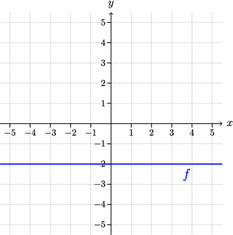
Da \(f\) ikke skærer \(x\)-aksen, har \(f\) ingen nulpunkter.
Da grafen er under \(x\)-aksen for alle \(x\)-værdier, er det simpelt at lave en fortegnsundersøgelse. Vi skriver blot:
Øvelse 2.4.3
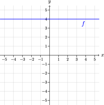
Lad \(f(x)=4\).
-
a) Bestem \(f(-3)\).
-
b) Tegn grafen for \(f\).
-
c) Bestem nulpunkter for \(f\).
-
d) Lav en fortegnsundersøgelse for \(f\).
Øvelse 2.4.4 ()
Ifølge definitionen er et nulpunkt en \(x\)-værdi med en funktionsværdi på nul.
2.4.4
-
a) Vi ved, at \(y\)-værdierne på grafen er det samme som funktionsværdierne for \(f\), så hvis funktionsværdien er nul, er \(y\) nul, hvilket betyder, at
vi har fat i et punkt, som ligger på \(x\)-aksen.
Nulpunkter og fortegnsundersøgelse ved beregning
Man beregner nulpunkterne ved at sætte \(f(x)=0\) og løse ligningen.
-
Eksempel 2.4.3
Vi ønsker at beregne nulpunkter for funktionen \(f(x)=2x-2\).
Vi sætter \(f(x)=0\) og løser ligningen:
\(\seteqnumber{0}{2.}{0}\)
\begin{align*}
f(x) &=0\\ 2x-2 &=0 && (\textrm {forskrift indsat})\\ 2x&=2\\ x &=1
\end{align*}
Altså har \(f(x)\) netop et nulpunkt, som er i \(x=1\).
Øvelse 2.4.5
Bestem ved beregning nulpunkterne for funktionerne:
-
a) \(f(x)=4x+2\)
-
b) \(g(x)=-x\)
-
c) \(f(x)=2(x+1)\)
2.4.5
-
a) \(x=-0{,}5\)
-
b) \(x=0\)
-
c) \(x=-1\)
Øvelse 2.4.6 ()
Bestem ved beregning nulpunkterne for funktionerne:
Når man har nulpunkterne, kan man lave fortegnsundersøgelsen ved at vælge nogle \(x\)-værdier omkring nulpunkterne, og indsætte dem i funktionen. Ud fra resultaterne kan man bestemme
fortegnsvariationen.
-
Eksempel 2.4.4
Lad \(f(x)=3x+6\).
Vi vil lave en fortegnsundersøgelse ved beregning.
Vi finder først nulpunkter:
\(\seteqnumber{0}{2.}{0}\)
\begin{align*}
f(x) & =0\\ 3x+6 & =0\\ 3x&=-6\\x&=-2
\end{align*}
Funktionen har altså nulpunkt i \(x=-2\). Vi vælger først en \(x\)-værdi til venstre for nulpunktet (dvs. en \(x\)-værdi, som er mindre end \(-2\)). Vi tager \(x=-3\), men vi kunne også have taget \(x=-4\), \(x=-5\) osv. Vi
vælger så en \(x\)-værdi til højre for nulpunktet. Her tager vi \(x=0\). Vi regner nu de tilhørende funktionsværdier:
\[f(-3)=3\cdot (-3)+6=-3\quad \text {og}\quad f(0)=3\cdot 0+6=6\]
Vi skriver nulpunktet og de to funktionsværdier ind i et sildeben.
\(\begin {array} {| c | c | c | c |} \hline x & -3 & -2 & 0\\ \hline f(x) & -3 &0 & 6 \\ \hline \end {array}\)
Vi kan se, at funktionsværdierne er negative til venstre for \(x=-2\) og positive til højre for \(x=-2\), så det giver os fortegnsvariationen:
| . |
|---|
| \(f\) er negativ i \(]-\infty ;-2[\) |
| \(f\) er positiv i \(]-2;\infty [\) |
| \(f\) er nul, når \(x=-2\) |
Metoden fra eksemplet virker på alle funktioner, som har en sammenhængende graf. Indtil videre kan du gå ud fra, at grafen er sammenhængende, når du skal regne fortegnsvariationen.
Øvelse 2.4.7
Lad \(f(x)=-0{,}5x+2\)
-
Eksempel 2.4.5
Vi vil lave en fortegnsundersøgelse for funktionen med forskriften \(f(x)=x^2-6x+8\).
Vi skal starte med at bestemme nulpunkter, men desværre er det først senere du lærer, hvordan man beregner nulpunkter for den slags funktioner. Så jeg vil være flink og forære dig nulpunkterne, som er i \(x=2\) og \(x=4\). Hvis
du føler for det, kan du sætte dem ind i forskriften og tjekke, at jeg ikke binder dig noget på ærmet.
Vi vælger nu nogle \(x\)-værdier, som omgiver nulpunkterne. Vi vælger \(x=0\), \(x=3\) og \(x=5\):
\(\begin {array} {| c | c | c | c | c | c |} \hline x & 0 & 2 & 3 & 4 & 5\\ \hline f(x) & & 0 & & 0 & \\ \hline \end {array}\)
Vi regner nu de tilhørende funktionsværdier:
\(\begin {array} {| c | c | c | c | c | c |} \hline x & 0 & 2 & 3 & 4 & 5 \\ \hline f(x) & 8 & 0 & -1 & 0 & 3 \\ \hline \end {array}\)
Vi kan nu opskrive fortegnsvariationen:
| . |
|---|
| \(f\) er positiv i \(]-\infty ;2[\) og \(]4;\infty [\) |
| \(f\) er negativ i \(]2;4[\) |
| \(f\) er nul, når \(x=2\) og \(x=4\) |
Øvelse 2.4.8
Lad \(f(x)=x^3-3x^2+4\).
Funktionen \(f\) har netop to nulpunkter: \(x=-1\) og \(x=2\).