MATHHX A
\(\newcommand{\footnotename}{footnote}\)
\(\def \LWRfootnote {1}\)
\(\newcommand {\footnote }[2][\LWRfootnote ]{{}^{\mathrm {#1}}}\)
\(\newcommand {\footnotemark }[1][\LWRfootnote ]{{}^{\mathrm {#1}}}\)
\(\let \LWRorighspace \hspace \)
\(\renewcommand {\hspace }{\ifstar \LWRorighspace \LWRorighspace }\)
\(\newcommand {\TextOrMath }[2]{#2}\)
\(\newcommand {\mathnormal }[1]{{#1}}\)
\(\newcommand \ensuremath [1]{#1}\)
\(\newcommand {\LWRframebox }[2][]{\fbox {#2}} \newcommand {\framebox }[1][]{\LWRframebox } \)
\(\newcommand {\setlength }[2]{}\)
\(\newcommand {\addtolength }[2]{}\)
\(\newcommand {\setcounter }[2]{}\)
\(\newcommand {\addtocounter }[2]{}\)
\(\newcommand {\arabic }[1]{}\)
\(\newcommand {\number }[1]{}\)
\(\newcommand {\noalign }[1]{\text {#1}\notag \\}\)
\(\newcommand {\cline }[1]{}\)
\(\newcommand {\directlua }[1]{\text {(directlua)}}\)
\(\newcommand {\luatexdirectlua }[1]{\text {(directlua)}}\)
\(\newcommand {\protect }{}\)
\(\def \LWRabsorbnumber #1 {}\)
\(\def \LWRabsorbquotenumber "#1 {}\)
\(\newcommand {\LWRabsorboption }[1][]{}\)
\(\newcommand {\LWRabsorbtwooptions }[1][]{\LWRabsorboption }\)
\(\def \mathchar {\ifnextchar "\LWRabsorbquotenumber \LWRabsorbnumber }\)
\(\def \mathcode #1={\mathchar }\)
\(\let \delcode \mathcode \)
\(\let \delimiter \mathchar \)
\(\def \oe {\unicode {x0153}}\)
\(\def \OE {\unicode {x0152}}\)
\(\def \ae {\unicode {x00E6}}\)
\(\def \AE {\unicode {x00C6}}\)
\(\def \aa {\unicode {x00E5}}\)
\(\def \AA {\unicode {x00C5}}\)
\(\def \o {\unicode {x00F8}}\)
\(\def \O {\unicode {x00D8}}\)
\(\def \l {\unicode {x0142}}\)
\(\def \L {\unicode {x0141}}\)
\(\def \ss {\unicode {x00DF}}\)
\(\def \SS {\unicode {x1E9E}}\)
\(\def \dag {\unicode {x2020}}\)
\(\def \ddag {\unicode {x2021}}\)
\(\def \P {\unicode {x00B6}}\)
\(\def \copyright {\unicode {x00A9}}\)
\(\def \pounds {\unicode {x00A3}}\)
\(\let \LWRref \ref \)
\(\renewcommand {\ref }{\ifstar \LWRref \LWRref }\)
\( \newcommand {\multicolumn }[3]{#3}\)
\(\require {textcomp}\)
\(\require {colortbl}\)
\(\let \LWRorigcolumncolor \columncolor \)
\(\renewcommand {\columncolor }[2][named]{\LWRorigcolumncolor [#1]{#2}\LWRabsorbtwooptions }\)
\(\let \LWRorigrowcolor \rowcolor \)
\(\renewcommand {\rowcolor }[2][named]{\LWRorigrowcolor [#1]{#2}\LWRabsorbtwooptions }\)
\(\let \LWRorigcellcolor \cellcolor \)
\(\renewcommand {\cellcolor }[2][named]{\LWRorigcellcolor [#1]{#2}\LWRabsorbtwooptions }\)
\(\newcommand {\tothe }[1]{^{#1}}\)
\(\newcommand {\raiseto }[2]{{#2}^{#1}}\)
\(\newcommand {\LWRsiunitxEND }{}\)
\(\def \LWRsiunitxang #1;#2;#3;#4\LWRsiunitxEND {\ifblank {#1}{}{\num {#1}\degree }\ifblank {#2}{}{\num {#2}^{\unicode {x2032}}}\ifblank {#3}{}{\num {#3}^{\unicode {x2033}}}}\)
\(\newcommand {\ang }[2][]{\LWRsiunitxang #2;;;\LWRsiunitxEND }\)
\(\def \LWRsiunitxdistribunit {}\)
\(\newcommand {\LWRsiunitxENDTWO }{}\)
\(\def \LWRsiunitxprintdecimalsubtwo #1,#2,#3\LWRsiunitxENDTWO {\ifblank {#1}{0}{\mathrm {#1}}\ifblank {#2}{}{{\LWRsiunitxdecimal }\mathrm {#2}}}\)
\(\def \LWRsiunitxprintdecimalsub #1.#2.#3\LWRsiunitxEND {\LWRsiunitxprintdecimalsubtwo #1,,\LWRsiunitxENDTWO \ifblank {#2}{}{{\LWRsiunitxdecimal }\LWRsiunitxprintdecimalsubtwo
#2,,\LWRsiunitxENDTWO }}\)
\(\newcommand {\LWRsiunitxprintdecimal }[1]{\LWRsiunitxprintdecimalsub #1...\LWRsiunitxEND }\)
\(\def \LWRsiunitxnumplus #1+#2+#3\LWRsiunitxEND {\ifblank {#2}{\LWRsiunitxprintdecimal {#1}}{\ifblank {#1}{\LWRsiunitxprintdecimal {#2}}{\LWRsiunitxprintdecimal {#1}\unicode
{x02B}\LWRsiunitxprintdecimal {#2}}}\LWRsiunitxdistribunit }\)
\(\def \LWRsiunitxnumminus #1-#2-#3\LWRsiunitxEND {\ifblank {#2}{\LWRsiunitxnumplus #1+++\LWRsiunitxEND }{\ifblank {#1}{}{\LWRsiunitxprintdecimal {#1}}\unicode {x02212}\LWRsiunitxprintdecimal
{#2}\LWRsiunitxdistribunit }}\)
\(\def \LWRsiunitxnumpmmacro #1\pm #2\pm #3\LWRsiunitxEND {\ifblank {#2}{\LWRsiunitxnumminus #1---\LWRsiunitxEND }{\LWRsiunitxprintdecimal {#1}\unicode {x0B1}\LWRsiunitxprintdecimal
{#2}\LWRsiunitxdistribunit }}\)
\(\def \LWRsiunitxnumpm #1+-#2+-#3\LWRsiunitxEND {\ifblank {#2}{\LWRsiunitxnumpmmacro #1\pm \pm \pm \LWRsiunitxEND }{\LWRsiunitxprintdecimal {#1}\unicode {x0B1}\LWRsiunitxprintdecimal
{#2}\LWRsiunitxdistribunit }}\)
\(\newcommand {\LWRsiunitxnumscientific }[2]{\ifblank {#1}{}{\ifstrequal {#1}{-}{-}{\LWRsiunitxprintdecimal {#1}\times }}10^{\LWRsiunitxprintdecimal {#2}}\LWRsiunitxdistribunit }\)
\(\def \LWRsiunitxnumD #1D#2D#3\LWRsiunitxEND {\ifblank {#2}{\LWRsiunitxnumpm #1+-+-\LWRsiunitxEND }{\mathrm {\LWRsiunitxnumscientific {#1}{#2}}}}\)
\(\def \LWRsiunitxnumd #1d#2d#3\LWRsiunitxEND {\ifblank {#2}{\LWRsiunitxnumD #1DDD\LWRsiunitxEND }{\mathrm {\LWRsiunitxnumscientific {#1}{#2}}}}\)
\(\def \LWRsiunitxnumE #1E#2E#3\LWRsiunitxEND {\ifblank {#2}{\LWRsiunitxnumd #1ddd\LWRsiunitxEND }{\mathrm {\LWRsiunitxnumscientific {#1}{#2}}}}\)
\(\def \LWRsiunitxnume #1e#2e#3\LWRsiunitxEND {\ifblank {#2}{\LWRsiunitxnumE #1EEE\LWRsiunitxEND }{\mathrm {\LWRsiunitxnumscientific {#1}{#2}}}}\)
\(\def \LWRsiunitxnumx #1x#2x#3x#4\LWRsiunitxEND {\ifblank {#2}{\LWRsiunitxnume #1eee\LWRsiunitxEND }{\ifblank {#3}{\LWRsiunitxnume #1eee\LWRsiunitxEND \times \LWRsiunitxnume
#2eee\LWRsiunitxEND }{\LWRsiunitxnume #1eee\LWRsiunitxEND \times \LWRsiunitxnume #2eee\LWRsiunitxEND \times \LWRsiunitxnume #3eee\LWRsiunitxEND }}}\)
\(\newcommand {\num }[2][]{\LWRsiunitxnumx #2xxxxx\LWRsiunitxEND }\)
\(\newcommand {\si }[2][]{\mathrm {\gsubstitute {#2}{~}{\,}}}\)
\(\def \LWRsiunitxSIopt #1[#2]#3{\def \LWRsiunitxdistribunit {\,\si {#3}}{#2}\num {#1}\def \LWRsiunitxdistribunit {}}\)
\(\newcommand {\LWRsiunitxSI }[2]{\def \LWRsiunitxdistribunit {\,\si {#2}}\num {#1}\def \LWRsiunitxdistribunit {}}\)
\(\newcommand {\SI }[2][]{\ifnextchar [{\LWRsiunitxSIopt {#2}}{\LWRsiunitxSI {#2}}}\)
\(\newcommand {\numlist }[2][]{\text {#2}}\)
\(\newcommand {\numrange }[3][]{\num {#2}\ \LWRsiunitxrangephrase \ \num {#3}}\)
\(\newcommand {\SIlist }[3][]{\text {#2}\,\si {#3}}\)
\(\newcommand {\SIrange }[4][]{\num {#2}\,#4\ \LWRsiunitxrangephrase \ \num {#3}\,#4}\)
\(\newcommand {\tablenum }[2][]{\mathrm {#2}}\)
\(\newcommand {\ampere }{\mathrm {A}}\)
\(\newcommand {\candela }{\mathrm {cd}}\)
\(\newcommand {\kelvin }{\mathrm {K}}\)
\(\newcommand {\kilogram }{\mathrm {kg}}\)
\(\newcommand {\metre }{\mathrm {m}}\)
\(\newcommand {\mole }{\mathrm {mol}}\)
\(\newcommand {\second }{\mathrm {s}}\)
\(\newcommand {\becquerel }{\mathrm {Bq}}\)
\(\newcommand {\degreeCelsius }{\unicode {x2103}}\)
\(\newcommand {\coulomb }{\mathrm {C}}\)
\(\newcommand {\farad }{\mathrm {F}}\)
\(\newcommand {\gray }{\mathrm {Gy}}\)
\(\newcommand {\hertz }{\mathrm {Hz}}\)
\(\newcommand {\henry }{\mathrm {H}}\)
\(\newcommand {\joule }{\mathrm {J}}\)
\(\newcommand {\katal }{\mathrm {kat}}\)
\(\newcommand {\lumen }{\mathrm {lm}}\)
\(\newcommand {\lux }{\mathrm {lx}}\)
\(\newcommand {\newton }{\mathrm {N}}\)
\(\newcommand {\ohm }{\mathrm {\Omega }}\)
\(\newcommand {\pascal }{\mathrm {Pa}}\)
\(\newcommand {\radian }{\mathrm {rad}}\)
\(\newcommand {\siemens }{\mathrm {S}}\)
\(\newcommand {\sievert }{\mathrm {Sv}}\)
\(\newcommand {\steradian }{\mathrm {sr}}\)
\(\newcommand {\tesla }{\mathrm {T}}\)
\(\newcommand {\volt }{\mathrm {V}}\)
\(\newcommand {\watt }{\mathrm {W}}\)
\(\newcommand {\weber }{\mathrm {Wb}}\)
\(\newcommand {\day }{\mathrm {d}}\)
\(\newcommand {\degree }{\mathrm {^\circ }}\)
\(\newcommand {\hectare }{\mathrm {ha}}\)
\(\newcommand {\hour }{\mathrm {h}}\)
\(\newcommand {\litre }{\mathrm {l}}\)
\(\newcommand {\liter }{\mathrm {L}}\)
\(\newcommand {\arcminute }{^\prime }\)
\(\newcommand {\minute }{\mathrm {min}}\)
\(\newcommand {\arcsecond }{^{\prime \prime }}\)
\(\newcommand {\tonne }{\mathrm {t}}\)
\(\newcommand {\astronomicalunit }{au}\)
\(\newcommand {\atomicmassunit }{u}\)
\(\newcommand {\bohr }{\mathit {a}_0}\)
\(\newcommand {\clight }{\mathit {c}_0}\)
\(\newcommand {\dalton }{\mathrm {D}_\mathrm {a}}\)
\(\newcommand {\electronmass }{\mathit {m}_{\mathrm {e}}}\)
\(\newcommand {\electronvolt }{\mathrm {eV}}\)
\(\newcommand {\elementarycharge }{\mathit {e}}\)
\(\newcommand {\hartree }{\mathit {E}_{\mathrm {h}}}\)
\(\newcommand {\planckbar }{\mathit {\unicode {x210F}}}\)
\(\newcommand {\angstrom }{\mathrm {\unicode {x212B}}}\)
\(\let \LWRorigbar \bar \)
\(\newcommand {\barn }{\mathrm {b}}\)
\(\newcommand {\bel }{\mathrm {B}}\)
\(\newcommand {\decibel }{\mathrm {dB}}\)
\(\newcommand {\knot }{\mathrm {kn}}\)
\(\newcommand {\mmHg }{\mathrm {mmHg}}\)
\(\newcommand {\nauticalmile }{\mathrm {M}}\)
\(\newcommand {\neper }{\mathrm {Np}}\)
\(\newcommand {\yocto }{\mathrm {y}}\)
\(\newcommand {\zepto }{\mathrm {z}}\)
\(\newcommand {\atto }{\mathrm {a}}\)
\(\newcommand {\femto }{\mathrm {f}}\)
\(\newcommand {\pico }{\mathrm {p}}\)
\(\newcommand {\nano }{\mathrm {n}}\)
\(\newcommand {\micro }{\mathrm {\unicode {x00B5}}}\)
\(\newcommand {\milli }{\mathrm {m}}\)
\(\newcommand {\centi }{\mathrm {c}}\)
\(\newcommand {\deci }{\mathrm {d}}\)
\(\newcommand {\deca }{\mathrm {da}}\)
\(\newcommand {\hecto }{\mathrm {h}}\)
\(\newcommand {\kilo }{\mathrm {k}}\)
\(\newcommand {\mega }{\mathrm {M}}\)
\(\newcommand {\giga }{\mathrm {G}}\)
\(\newcommand {\tera }{\mathrm {T}}\)
\(\newcommand {\peta }{\mathrm {P}}\)
\(\newcommand {\exa }{\mathrm {E}}\)
\(\newcommand {\zetta }{\mathrm {Z}}\)
\(\newcommand {\yotta }{\mathrm {Y}}\)
\(\newcommand {\percent }{\mathrm {\%}}\)
\(\newcommand {\meter }{\mathrm {m}}\)
\(\newcommand {\metre }{\mathrm {m}}\)
\(\newcommand {\gram }{\mathrm {g}}\)
\(\newcommand {\kg }{\kilo \gram }\)
\(\newcommand {\of }[1]{_{\mathrm {#1}}}\)
\(\newcommand {\squared }{^2}\)
\(\newcommand {\square }[1]{\mathrm {#1}^2}\)
\(\newcommand {\cubed }{^3}\)
\(\newcommand {\cubic }[1]{\mathrm {#1}^3}\)
\(\newcommand {\per }{\,\mathrm {/}}\)
\(\newcommand {\celsius }{\unicode {x2103}}\)
\(\newcommand {\fg }{\femto \gram }\)
\(\newcommand {\pg }{\pico \gram }\)
\(\newcommand {\ng }{\nano \gram }\)
\(\newcommand {\ug }{\micro \gram }\)
\(\newcommand {\mg }{\milli \gram }\)
\(\newcommand {\g }{\gram }\)
\(\newcommand {\kg }{\kilo \gram }\)
\(\newcommand {\amu }{\mathrm {u}}\)
\(\newcommand {\nm }{\nano \metre }\)
\(\newcommand {\um }{\micro \metre }\)
\(\newcommand {\mm }{\milli \metre }\)
\(\newcommand {\cm }{\centi \metre }\)
\(\newcommand {\dm }{\deci \metre }\)
\(\newcommand {\m }{\metre }\)
\(\newcommand {\km }{\kilo \metre }\)
\(\newcommand {\as }{\atto \second }\)
\(\newcommand {\fs }{\femto \second }\)
\(\newcommand {\ps }{\pico \second }\)
\(\newcommand {\ns }{\nano \second }\)
\(\newcommand {\us }{\micro \second }\)
\(\newcommand {\ms }{\milli \second }\)
\(\newcommand {\s }{\second }\)
\(\newcommand {\fmol }{\femto \mol }\)
\(\newcommand {\pmol }{\pico \mol }\)
\(\newcommand {\nmol }{\nano \mol }\)
\(\newcommand {\umol }{\micro \mol }\)
\(\newcommand {\mmol }{\milli \mol }\)
\(\newcommand {\mol }{\mol }\)
\(\newcommand {\kmol }{\kilo \mol }\)
\(\newcommand {\pA }{\pico \ampere }\)
\(\newcommand {\nA }{\nano \ampere }\)
\(\newcommand {\uA }{\micro \ampere }\)
\(\newcommand {\mA }{\milli \ampere }\)
\(\newcommand {\A }{\ampere }\)
\(\newcommand {\kA }{\kilo \ampere }\)
\(\newcommand {\ul }{\micro \litre }\)
\(\newcommand {\ml }{\milli \litre }\)
\(\newcommand {\l }{\litre }\)
\(\newcommand {\hl }{\hecto \litre }\)
\(\newcommand {\uL }{\micro \liter }\)
\(\newcommand {\mL }{\milli \liter }\)
\(\newcommand {\L }{\liter }\)
\(\newcommand {\hL }{\hecto \liter }\)
\(\newcommand {\mHz }{\milli \hertz }\)
\(\newcommand {\Hz }{\hertz }\)
\(\newcommand {\kHz }{\kilo \hertz }\)
\(\newcommand {\MHz }{\mega \hertz }\)
\(\newcommand {\GHz }{\giga \hertz }\)
\(\newcommand {\THz }{\tera \hertz }\)
\(\newcommand {\mN }{\milli \newton }\)
\(\newcommand {\N }{\newton }\)
\(\newcommand {\kN }{\kilo \newton }\)
\(\newcommand {\MN }{\mega \newton }\)
\(\newcommand {\Pa }{\pascal }\)
\(\newcommand {\kPa }{\kilo \pascal }\)
\(\newcommand {\MPa }{\mega \pascal }\)
\(\newcommand {\GPa }{\giga \pascal }\)
\(\newcommand {\mohm }{\milli \ohm }\)
\(\newcommand {\kohm }{\kilo \ohm }\)
\(\newcommand {\Mohm }{\mega \ohm }\)
\(\newcommand {\pV }{\pico \volt }\)
\(\newcommand {\nV }{\nano \volt }\)
\(\newcommand {\uV }{\micro \volt }\)
\(\newcommand {\mV }{\milli \volt }\)
\(\newcommand {\V }{\volt }\)
\(\newcommand {\kV }{\kilo \volt }\)
\(\newcommand {\W }{\watt }\)
\(\newcommand {\uW }{\micro \watt }\)
\(\newcommand {\mW }{\milli \watt }\)
\(\newcommand {\kW }{\kilo \watt }\)
\(\newcommand {\MW }{\mega \watt }\)
\(\newcommand {\GW }{\giga \watt }\)
\(\newcommand {\J }{\joule }\)
\(\newcommand {\uJ }{\micro \joule }\)
\(\newcommand {\mJ }{\milli \joule }\)
\(\newcommand {\kJ }{\kilo \joule }\)
\(\newcommand {\eV }{\electronvolt }\)
\(\newcommand {\meV }{\milli \electronvolt }\)
\(\newcommand {\keV }{\kilo \electronvolt }\)
\(\newcommand {\MeV }{\mega \electronvolt }\)
\(\newcommand {\GeV }{\giga \electronvolt }\)
\(\newcommand {\TeV }{\tera \electronvolt }\)
\(\newcommand {\kWh }{\kilo \watt \hour }\)
\(\newcommand {\F }{\farad }\)
\(\newcommand {\fF }{\femto \farad }\)
\(\newcommand {\pF }{\pico \farad }\)
\(\newcommand {\K }{\mathrm {K}}\)
\(\newcommand {\dB }{\mathrm {dB}}\)
\(\newcommand {\kibi }{\mathrm {Ki}}\)
\(\newcommand {\mebi }{\mathrm {Mi}}\)
\(\newcommand {\gibi }{\mathrm {Gi}}\)
\(\newcommand {\tebi }{\mathrm {Ti}}\)
\(\newcommand {\pebi }{\mathrm {Pi}}\)
\(\newcommand {\exbi }{\mathrm {Ei}}\)
\(\newcommand {\zebi }{\mathrm {Zi}}\)
\(\newcommand {\yobi }{\mathrm {Yi}}\)
\(\let \unit \si \)
\(\let \qty \SI \)
\(\let \qtylist \SIlist \)
\(\let \qtyrange \SIrange \)
\(\let \numproduct \num \)
\(\let \qtyproduct \SI \)
\(\let \complexnum \num \)
\(\newcommand {\complexqty }[3][]{(\complexnum {#2})\si {#3}}\)
\(\newcommand {\mleft }{\left }\)
\(\newcommand {\mright }{\right }\)
\(\newcommand {\mleftright }{}\)
\(\newcommand {\mleftrightrestore }{}\)
\(\require {gensymb}\)
\(\newcommand {\intertext }[1]{\text {#1}\notag \\}\)
\(\let \Hat \hat \)
\(\let \Check \check \)
\(\let \Tilde \tilde \)
\(\let \Acute \acute \)
\(\let \Grave \grave \)
\(\let \Dot \dot \)
\(\let \Ddot \ddot \)
\(\let \Breve \breve \)
\(\let \Bar \bar \)
\(\let \Vec \vec \)
\(\require {cancel}\)
\(\newcommand {\mathred }[1]{\textcolor [rgb]{1, 0, 0}{#1}}\)
\(\newcommand {\mathgreen }[1]{\textcolor [rgb]{0,0.5,0}{#1}}\)
\(\newcommand {\mathblue }[1]{\textcolor [rgb]{0,0,1}{#1}}\)
\(\newcommand {\mathorange }[1]{\textcolor [rgb]{1,0.5,0}{#1}}\)
\(\newcommand {\mathmagenta }[1]{\textcolor [cmyk]{0, 1, 1, 0.33}{#1}}\)
\( \newcommand \ccancel [2][red]{\renewcommand \CancelColor {\color {#1}}\cancel {#2}} \)
\(\newcommand {\Dom }{\operatorname {Dom}}\)
\(\newcommand {\Ran }{\operatorname {Ran}}\)
\(\newcommand {\Dm }{\operatorname {Dm}}\)
\(\newcommand {\Vm }{\operatorname {Vm}}\)
\(\newcommand {\Var }{\operatorname {Var}}\)
\(\newcommand {\SD }{\operatorname {SD}}\)
\(\newcommand {\ExV }{\operatorname {E}}\)
\(\newcommand {\opointtext }{\textcolor {blue}{\circ }}\)
\(\newcommand {\cpointtext }{\textcolor {blue}{\bullet }}\)
\(\newcommand {\vectwo }[2]{\begin {pmatrix} #1 \\ #2 \end {pmatrix}}\)
\(\newcommand {\tcbset }[1]{}\)
\(\newcommand {\tcbsetforeverylayer }[1]{}\)
\(\newcommand {\tcbox }[2][]{\boxed {\text {#2}}}\)
\(\newcommand {\tcboxfit }[2][]{\boxed {#2}}\)
\(\newcommand {\tcblower }{}\)
\(\newcommand {\tcbline }{}\)
\(\newcommand {\tcbtitle }{}\)
\(\newcommand {\tcbsubtitle [2][]{\mathrm {#2}}}\)
\(\newcommand {\tcboxmath }[2][]{\boxed {#2}}\)
\(\newcommand {\tcbhighmath }[2][]{\boxed {#2}}\)
\(\newcommand {\toprule }[1][]{\hline }\)
\(\let \midrule \toprule \)
\(\let \bottomrule \toprule \)
\(\def \LWRbooktabscmidruleparen (#1)#2{}\)
\(\newcommand {\LWRbooktabscmidrulenoparen }[1]{}\)
\(\newcommand {\cmidrule }[1][]{\ifnextchar (\LWRbooktabscmidruleparen \LWRbooktabscmidrulenoparen }\)
\(\newcommand {\morecmidrules }{}\)
\(\newcommand {\specialrule }[3]{\hline }\)
\(\newcommand {\addlinespace }[1][]{}\)
\(\def \LWRsiunitxrangephrase {\TextOrMath { }{\ }\protect \mbox {to (numerical range)}\TextOrMath { }{\ }}\)
\(\def \LWRsiunitxdecimal {.}\)
5.6 Normalfordelte observationssæt
Lad os lege, at vi plukker æbler fra en æbleplantage. Her mener jeg frugten æble og ikke computere af mærket ”Apple”. Vægten af et æble vil variere fra æble til æble, og derfor kan vægten af et tilfældigt æble beskrives med en
stokastisk variabel \(X\). Vi antager nu, at vægten \(X\), målt i gram, er normalfordelt:
\[X\sim N(100,20)\]
Lad os sige, at vi plukker \(500\) æbler og laver et histogram over æblernes vægt. Hvordan vil vi forvente, at histogrammet ser ud? Ja, det må jo ligne tæthedsfunktionen for \(X\), fordi arealerne af søjlerne i histogrammet viser
frekvenserne, og frekvenserne må jo svare nogenlunde til sandsynlighederne, når stikprøven er stor. Altså, hvis der f.eks. er \(15\%\) sandsynlighed for, at et æble vejer mellem \(110\) og \(120\) gram, så vil vi jo forvente, at
\(15\%\) af de æbler, vi plukker, vil veje mellem \(110\) og \(120\) gram. Jeg har simuleret \(500\) æbler ved at generere \(500\) værdier fra fordelingen \(N(100,20)\):
Jeg tilføjer nu tæthedsfunktionen for \(X\sim N(100,20)\):
Vi ser, at histogrammet følger tæthedsfunktionen som forventet.
Vi skal nu se, hvordan kan man undersøge, om et givet observationssæt følger en normalfordeling. Vi vil tage udgangspunkt i det første observationssæt i filen her. Vi skal også bruge Excel-arket fra WordMat statistik. Hvis du har glemt, hvordan man åbner det, så find WordMat-afsnittet i statistikkapitlet i b-bogen.
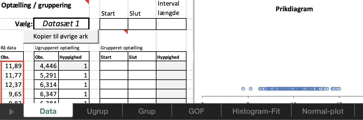
Vi starter med at åbne observationssættet og kopiere data fra det første observationssæt ind i WordMat-statistik som vist her:
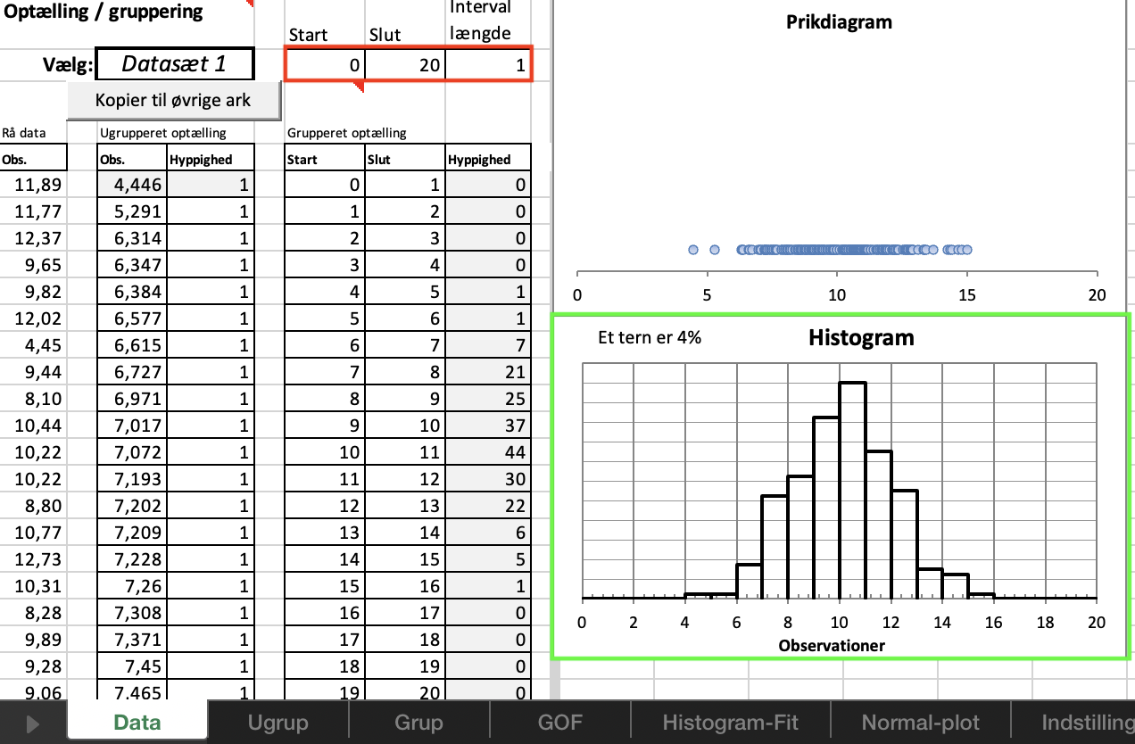
Vi vil først lave et histogram og se, om det ser nogenlunde normalfordelt ud. Vi får histogrammet ved at gruppere data. Vi kan se, at værdierne ligger imellem 0 og 20, så vi vælger det som grænser. Vi sætter intervalbredden til 1, så
vi får 20 intervaller. Generelt er det en god idé at lave histogrammet med 10 – 20 intervaller:
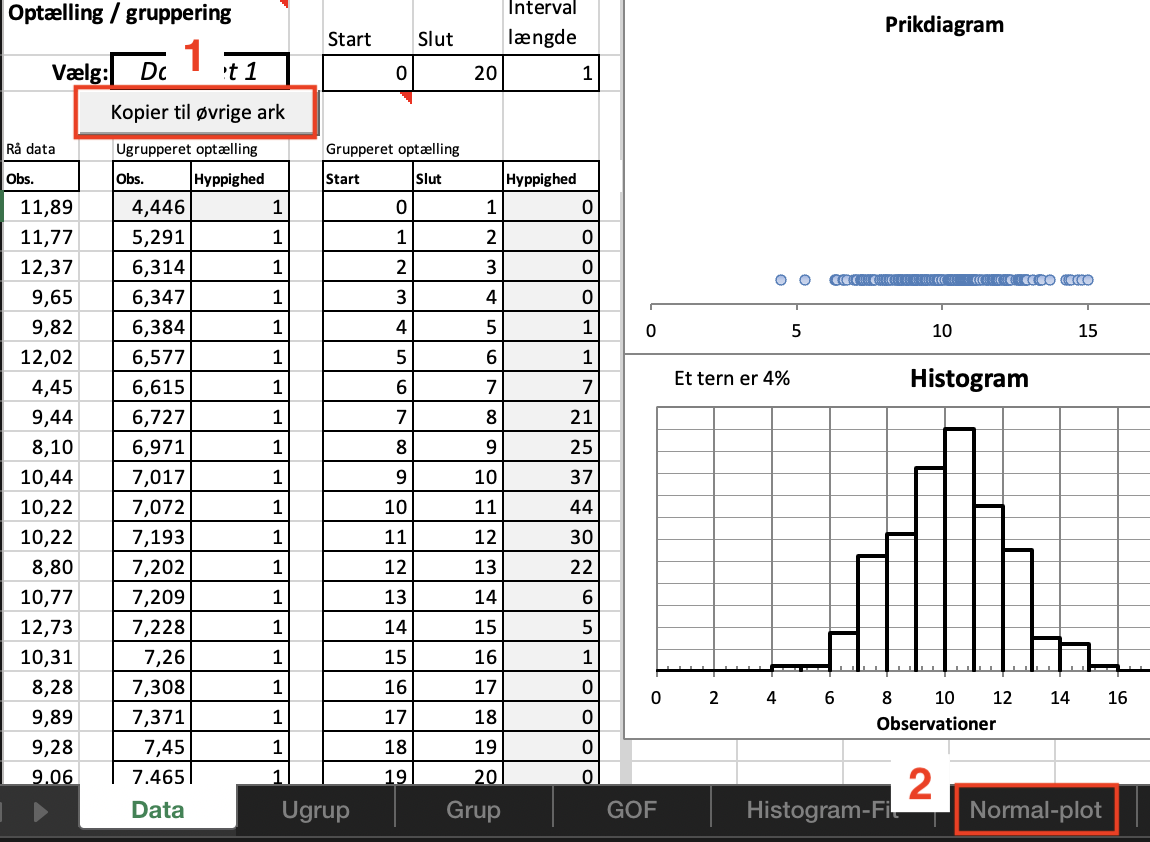
Vi ser, at histogrammet tilnærmelsesvist har form som tæthedsfunktionen for en normalfordeling. Det tyder på, at data godt kunne være normalfordelt. Vi kan tjekke dette lidt mere præcist ved at klikke ”Kopier til øvrige ark” og
vælge ”Normal-plot” i bunden:
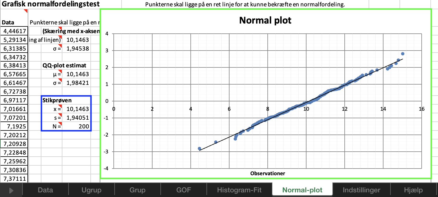
Det giver os:
Plottet i den grønne boks er et eksempel på det, man kalder et QQ-plot. Vi skal ikke gå i detaljer med, hvordan det er konstrueret, men jeg kan fortælle, at hvis punkterne ligger
tilnærmelsesvist på en linje, så er data tilnærmelsesvist normalfordelt. Vi ser, at dette er opfyldt i vores tilfælde, så data er tilnærmelsesvist normalfordelt. I den blå boks ses tallene \(x=1{,}98\) og \(s=10{,}1\). De to tal er
estimater for hhv. middelværdien og standardafvigelsen. Der er flere måder at estimere dem på og over den blå boks ses to alternative estimater. Der er fordele og ulemper ved de forskellige metoder, men det må blive en anden god
gang, at vi kigger på det.