MATHHX A
\(\newcommand{\footnotename}{footnote}\)
\(\def \LWRfootnote {1}\)
\(\newcommand {\footnote }[2][\LWRfootnote ]{{}^{\mathrm {#1}}}\)
\(\newcommand {\footnotemark }[1][\LWRfootnote ]{{}^{\mathrm {#1}}}\)
\(\let \LWRorighspace \hspace \)
\(\renewcommand {\hspace }{\ifstar \LWRorighspace \LWRorighspace }\)
\(\newcommand {\TextOrMath }[2]{#2}\)
\(\newcommand {\mathnormal }[1]{{#1}}\)
\(\newcommand \ensuremath [1]{#1}\)
\(\newcommand {\LWRframebox }[2][]{\fbox {#2}} \newcommand {\framebox }[1][]{\LWRframebox } \)
\(\newcommand {\setlength }[2]{}\)
\(\newcommand {\addtolength }[2]{}\)
\(\newcommand {\setcounter }[2]{}\)
\(\newcommand {\addtocounter }[2]{}\)
\(\newcommand {\arabic }[1]{}\)
\(\newcommand {\number }[1]{}\)
\(\newcommand {\noalign }[1]{\text {#1}\notag \\}\)
\(\newcommand {\cline }[1]{}\)
\(\newcommand {\directlua }[1]{\text {(directlua)}}\)
\(\newcommand {\luatexdirectlua }[1]{\text {(directlua)}}\)
\(\newcommand {\protect }{}\)
\(\def \LWRabsorbnumber #1 {}\)
\(\def \LWRabsorbquotenumber "#1 {}\)
\(\newcommand {\LWRabsorboption }[1][]{}\)
\(\newcommand {\LWRabsorbtwooptions }[1][]{\LWRabsorboption }\)
\(\def \mathchar {\ifnextchar "\LWRabsorbquotenumber \LWRabsorbnumber }\)
\(\def \mathcode #1={\mathchar }\)
\(\let \delcode \mathcode \)
\(\let \delimiter \mathchar \)
\(\def \oe {\unicode {x0153}}\)
\(\def \OE {\unicode {x0152}}\)
\(\def \ae {\unicode {x00E6}}\)
\(\def \AE {\unicode {x00C6}}\)
\(\def \aa {\unicode {x00E5}}\)
\(\def \AA {\unicode {x00C5}}\)
\(\def \o {\unicode {x00F8}}\)
\(\def \O {\unicode {x00D8}}\)
\(\def \l {\unicode {x0142}}\)
\(\def \L {\unicode {x0141}}\)
\(\def \ss {\unicode {x00DF}}\)
\(\def \SS {\unicode {x1E9E}}\)
\(\def \dag {\unicode {x2020}}\)
\(\def \ddag {\unicode {x2021}}\)
\(\def \P {\unicode {x00B6}}\)
\(\def \copyright {\unicode {x00A9}}\)
\(\def \pounds {\unicode {x00A3}}\)
\(\let \LWRref \ref \)
\(\renewcommand {\ref }{\ifstar \LWRref \LWRref }\)
\( \newcommand {\multicolumn }[3]{#3}\)
\(\require {textcomp}\)
\(\require {colortbl}\)
\(\let \LWRorigcolumncolor \columncolor \)
\(\renewcommand {\columncolor }[2][named]{\LWRorigcolumncolor [#1]{#2}\LWRabsorbtwooptions }\)
\(\let \LWRorigrowcolor \rowcolor \)
\(\renewcommand {\rowcolor }[2][named]{\LWRorigrowcolor [#1]{#2}\LWRabsorbtwooptions }\)
\(\let \LWRorigcellcolor \cellcolor \)
\(\renewcommand {\cellcolor }[2][named]{\LWRorigcellcolor [#1]{#2}\LWRabsorbtwooptions }\)
\(\newcommand {\tothe }[1]{^{#1}}\)
\(\newcommand {\raiseto }[2]{{#2}^{#1}}\)
\(\newcommand {\LWRsiunitxEND }{}\)
\(\def \LWRsiunitxang #1;#2;#3;#4\LWRsiunitxEND {\ifblank {#1}{}{\num {#1}\degree }\ifblank {#2}{}{\num {#2}^{\unicode {x2032}}}\ifblank {#3}{}{\num {#3}^{\unicode {x2033}}}}\)
\(\newcommand {\ang }[2][]{\LWRsiunitxang #2;;;\LWRsiunitxEND }\)
\(\def \LWRsiunitxdistribunit {}\)
\(\newcommand {\LWRsiunitxENDTWO }{}\)
\(\def \LWRsiunitxprintdecimalsubtwo #1,#2,#3\LWRsiunitxENDTWO {\ifblank {#1}{0}{\mathrm {#1}}\ifblank {#2}{}{{\LWRsiunitxdecimal }\mathrm {#2}}}\)
\(\def \LWRsiunitxprintdecimalsub #1.#2.#3\LWRsiunitxEND {\LWRsiunitxprintdecimalsubtwo #1,,\LWRsiunitxENDTWO \ifblank {#2}{}{{\LWRsiunitxdecimal }\LWRsiunitxprintdecimalsubtwo
#2,,\LWRsiunitxENDTWO }}\)
\(\newcommand {\LWRsiunitxprintdecimal }[1]{\LWRsiunitxprintdecimalsub #1...\LWRsiunitxEND }\)
\(\def \LWRsiunitxnumplus #1+#2+#3\LWRsiunitxEND {\ifblank {#2}{\LWRsiunitxprintdecimal {#1}}{\ifblank {#1}{\LWRsiunitxprintdecimal {#2}}{\LWRsiunitxprintdecimal {#1}\unicode
{x02B}\LWRsiunitxprintdecimal {#2}}}\LWRsiunitxdistribunit }\)
\(\def \LWRsiunitxnumminus #1-#2-#3\LWRsiunitxEND {\ifblank {#2}{\LWRsiunitxnumplus #1+++\LWRsiunitxEND }{\ifblank {#1}{}{\LWRsiunitxprintdecimal {#1}}\unicode {x02212}\LWRsiunitxprintdecimal
{#2}\LWRsiunitxdistribunit }}\)
\(\def \LWRsiunitxnumpmmacro #1\pm #2\pm #3\LWRsiunitxEND {\ifblank {#2}{\LWRsiunitxnumminus #1---\LWRsiunitxEND }{\LWRsiunitxprintdecimal {#1}\unicode {x0B1}\LWRsiunitxprintdecimal
{#2}\LWRsiunitxdistribunit }}\)
\(\def \LWRsiunitxnumpm #1+-#2+-#3\LWRsiunitxEND {\ifblank {#2}{\LWRsiunitxnumpmmacro #1\pm \pm \pm \LWRsiunitxEND }{\LWRsiunitxprintdecimal {#1}\unicode {x0B1}\LWRsiunitxprintdecimal
{#2}\LWRsiunitxdistribunit }}\)
\(\newcommand {\LWRsiunitxnumscientific }[2]{\ifblank {#1}{}{\ifstrequal {#1}{-}{-}{\LWRsiunitxprintdecimal {#1}\times }}10^{\LWRsiunitxprintdecimal {#2}}\LWRsiunitxdistribunit }\)
\(\def \LWRsiunitxnumD #1D#2D#3\LWRsiunitxEND {\ifblank {#2}{\LWRsiunitxnumpm #1+-+-\LWRsiunitxEND }{\mathrm {\LWRsiunitxnumscientific {#1}{#2}}}}\)
\(\def \LWRsiunitxnumd #1d#2d#3\LWRsiunitxEND {\ifblank {#2}{\LWRsiunitxnumD #1DDD\LWRsiunitxEND }{\mathrm {\LWRsiunitxnumscientific {#1}{#2}}}}\)
\(\def \LWRsiunitxnumE #1E#2E#3\LWRsiunitxEND {\ifblank {#2}{\LWRsiunitxnumd #1ddd\LWRsiunitxEND }{\mathrm {\LWRsiunitxnumscientific {#1}{#2}}}}\)
\(\def \LWRsiunitxnume #1e#2e#3\LWRsiunitxEND {\ifblank {#2}{\LWRsiunitxnumE #1EEE\LWRsiunitxEND }{\mathrm {\LWRsiunitxnumscientific {#1}{#2}}}}\)
\(\def \LWRsiunitxnumx #1x#2x#3x#4\LWRsiunitxEND {\ifblank {#2}{\LWRsiunitxnume #1eee\LWRsiunitxEND }{\ifblank {#3}{\LWRsiunitxnume #1eee\LWRsiunitxEND \times \LWRsiunitxnume
#2eee\LWRsiunitxEND }{\LWRsiunitxnume #1eee\LWRsiunitxEND \times \LWRsiunitxnume #2eee\LWRsiunitxEND \times \LWRsiunitxnume #3eee\LWRsiunitxEND }}}\)
\(\newcommand {\num }[2][]{\LWRsiunitxnumx #2xxxxx\LWRsiunitxEND }\)
\(\newcommand {\si }[2][]{\mathrm {\gsubstitute {#2}{~}{\,}}}\)
\(\def \LWRsiunitxSIopt #1[#2]#3{\def \LWRsiunitxdistribunit {\,\si {#3}}{#2}\num {#1}\def \LWRsiunitxdistribunit {}}\)
\(\newcommand {\LWRsiunitxSI }[2]{\def \LWRsiunitxdistribunit {\,\si {#2}}\num {#1}\def \LWRsiunitxdistribunit {}}\)
\(\newcommand {\SI }[2][]{\ifnextchar [{\LWRsiunitxSIopt {#2}}{\LWRsiunitxSI {#2}}}\)
\(\newcommand {\numlist }[2][]{\text {#2}}\)
\(\newcommand {\numrange }[3][]{\num {#2}\ \LWRsiunitxrangephrase \ \num {#3}}\)
\(\newcommand {\SIlist }[3][]{\text {#2}\,\si {#3}}\)
\(\newcommand {\SIrange }[4][]{\num {#2}\,#4\ \LWRsiunitxrangephrase \ \num {#3}\,#4}\)
\(\newcommand {\tablenum }[2][]{\mathrm {#2}}\)
\(\newcommand {\ampere }{\mathrm {A}}\)
\(\newcommand {\candela }{\mathrm {cd}}\)
\(\newcommand {\kelvin }{\mathrm {K}}\)
\(\newcommand {\kilogram }{\mathrm {kg}}\)
\(\newcommand {\metre }{\mathrm {m}}\)
\(\newcommand {\mole }{\mathrm {mol}}\)
\(\newcommand {\second }{\mathrm {s}}\)
\(\newcommand {\becquerel }{\mathrm {Bq}}\)
\(\newcommand {\degreeCelsius }{\unicode {x2103}}\)
\(\newcommand {\coulomb }{\mathrm {C}}\)
\(\newcommand {\farad }{\mathrm {F}}\)
\(\newcommand {\gray }{\mathrm {Gy}}\)
\(\newcommand {\hertz }{\mathrm {Hz}}\)
\(\newcommand {\henry }{\mathrm {H}}\)
\(\newcommand {\joule }{\mathrm {J}}\)
\(\newcommand {\katal }{\mathrm {kat}}\)
\(\newcommand {\lumen }{\mathrm {lm}}\)
\(\newcommand {\lux }{\mathrm {lx}}\)
\(\newcommand {\newton }{\mathrm {N}}\)
\(\newcommand {\ohm }{\mathrm {\Omega }}\)
\(\newcommand {\pascal }{\mathrm {Pa}}\)
\(\newcommand {\radian }{\mathrm {rad}}\)
\(\newcommand {\siemens }{\mathrm {S}}\)
\(\newcommand {\sievert }{\mathrm {Sv}}\)
\(\newcommand {\steradian }{\mathrm {sr}}\)
\(\newcommand {\tesla }{\mathrm {T}}\)
\(\newcommand {\volt }{\mathrm {V}}\)
\(\newcommand {\watt }{\mathrm {W}}\)
\(\newcommand {\weber }{\mathrm {Wb}}\)
\(\newcommand {\day }{\mathrm {d}}\)
\(\newcommand {\degree }{\mathrm {^\circ }}\)
\(\newcommand {\hectare }{\mathrm {ha}}\)
\(\newcommand {\hour }{\mathrm {h}}\)
\(\newcommand {\litre }{\mathrm {l}}\)
\(\newcommand {\liter }{\mathrm {L}}\)
\(\newcommand {\arcminute }{^\prime }\)
\(\newcommand {\minute }{\mathrm {min}}\)
\(\newcommand {\arcsecond }{^{\prime \prime }}\)
\(\newcommand {\tonne }{\mathrm {t}}\)
\(\newcommand {\astronomicalunit }{au}\)
\(\newcommand {\atomicmassunit }{u}\)
\(\newcommand {\bohr }{\mathit {a}_0}\)
\(\newcommand {\clight }{\mathit {c}_0}\)
\(\newcommand {\dalton }{\mathrm {D}_\mathrm {a}}\)
\(\newcommand {\electronmass }{\mathit {m}_{\mathrm {e}}}\)
\(\newcommand {\electronvolt }{\mathrm {eV}}\)
\(\newcommand {\elementarycharge }{\mathit {e}}\)
\(\newcommand {\hartree }{\mathit {E}_{\mathrm {h}}}\)
\(\newcommand {\planckbar }{\mathit {\unicode {x210F}}}\)
\(\newcommand {\angstrom }{\mathrm {\unicode {x212B}}}\)
\(\let \LWRorigbar \bar \)
\(\newcommand {\barn }{\mathrm {b}}\)
\(\newcommand {\bel }{\mathrm {B}}\)
\(\newcommand {\decibel }{\mathrm {dB}}\)
\(\newcommand {\knot }{\mathrm {kn}}\)
\(\newcommand {\mmHg }{\mathrm {mmHg}}\)
\(\newcommand {\nauticalmile }{\mathrm {M}}\)
\(\newcommand {\neper }{\mathrm {Np}}\)
\(\newcommand {\yocto }{\mathrm {y}}\)
\(\newcommand {\zepto }{\mathrm {z}}\)
\(\newcommand {\atto }{\mathrm {a}}\)
\(\newcommand {\femto }{\mathrm {f}}\)
\(\newcommand {\pico }{\mathrm {p}}\)
\(\newcommand {\nano }{\mathrm {n}}\)
\(\newcommand {\micro }{\mathrm {\unicode {x00B5}}}\)
\(\newcommand {\milli }{\mathrm {m}}\)
\(\newcommand {\centi }{\mathrm {c}}\)
\(\newcommand {\deci }{\mathrm {d}}\)
\(\newcommand {\deca }{\mathrm {da}}\)
\(\newcommand {\hecto }{\mathrm {h}}\)
\(\newcommand {\kilo }{\mathrm {k}}\)
\(\newcommand {\mega }{\mathrm {M}}\)
\(\newcommand {\giga }{\mathrm {G}}\)
\(\newcommand {\tera }{\mathrm {T}}\)
\(\newcommand {\peta }{\mathrm {P}}\)
\(\newcommand {\exa }{\mathrm {E}}\)
\(\newcommand {\zetta }{\mathrm {Z}}\)
\(\newcommand {\yotta }{\mathrm {Y}}\)
\(\newcommand {\percent }{\mathrm {\%}}\)
\(\newcommand {\meter }{\mathrm {m}}\)
\(\newcommand {\metre }{\mathrm {m}}\)
\(\newcommand {\gram }{\mathrm {g}}\)
\(\newcommand {\kg }{\kilo \gram }\)
\(\newcommand {\of }[1]{_{\mathrm {#1}}}\)
\(\newcommand {\squared }{^2}\)
\(\newcommand {\square }[1]{\mathrm {#1}^2}\)
\(\newcommand {\cubed }{^3}\)
\(\newcommand {\cubic }[1]{\mathrm {#1}^3}\)
\(\newcommand {\per }{\,\mathrm {/}}\)
\(\newcommand {\celsius }{\unicode {x2103}}\)
\(\newcommand {\fg }{\femto \gram }\)
\(\newcommand {\pg }{\pico \gram }\)
\(\newcommand {\ng }{\nano \gram }\)
\(\newcommand {\ug }{\micro \gram }\)
\(\newcommand {\mg }{\milli \gram }\)
\(\newcommand {\g }{\gram }\)
\(\newcommand {\kg }{\kilo \gram }\)
\(\newcommand {\amu }{\mathrm {u}}\)
\(\newcommand {\nm }{\nano \metre }\)
\(\newcommand {\um }{\micro \metre }\)
\(\newcommand {\mm }{\milli \metre }\)
\(\newcommand {\cm }{\centi \metre }\)
\(\newcommand {\dm }{\deci \metre }\)
\(\newcommand {\m }{\metre }\)
\(\newcommand {\km }{\kilo \metre }\)
\(\newcommand {\as }{\atto \second }\)
\(\newcommand {\fs }{\femto \second }\)
\(\newcommand {\ps }{\pico \second }\)
\(\newcommand {\ns }{\nano \second }\)
\(\newcommand {\us }{\micro \second }\)
\(\newcommand {\ms }{\milli \second }\)
\(\newcommand {\s }{\second }\)
\(\newcommand {\fmol }{\femto \mol }\)
\(\newcommand {\pmol }{\pico \mol }\)
\(\newcommand {\nmol }{\nano \mol }\)
\(\newcommand {\umol }{\micro \mol }\)
\(\newcommand {\mmol }{\milli \mol }\)
\(\newcommand {\mol }{\mol }\)
\(\newcommand {\kmol }{\kilo \mol }\)
\(\newcommand {\pA }{\pico \ampere }\)
\(\newcommand {\nA }{\nano \ampere }\)
\(\newcommand {\uA }{\micro \ampere }\)
\(\newcommand {\mA }{\milli \ampere }\)
\(\newcommand {\A }{\ampere }\)
\(\newcommand {\kA }{\kilo \ampere }\)
\(\newcommand {\ul }{\micro \litre }\)
\(\newcommand {\ml }{\milli \litre }\)
\(\newcommand {\l }{\litre }\)
\(\newcommand {\hl }{\hecto \litre }\)
\(\newcommand {\uL }{\micro \liter }\)
\(\newcommand {\mL }{\milli \liter }\)
\(\newcommand {\L }{\liter }\)
\(\newcommand {\hL }{\hecto \liter }\)
\(\newcommand {\mHz }{\milli \hertz }\)
\(\newcommand {\Hz }{\hertz }\)
\(\newcommand {\kHz }{\kilo \hertz }\)
\(\newcommand {\MHz }{\mega \hertz }\)
\(\newcommand {\GHz }{\giga \hertz }\)
\(\newcommand {\THz }{\tera \hertz }\)
\(\newcommand {\mN }{\milli \newton }\)
\(\newcommand {\N }{\newton }\)
\(\newcommand {\kN }{\kilo \newton }\)
\(\newcommand {\MN }{\mega \newton }\)
\(\newcommand {\Pa }{\pascal }\)
\(\newcommand {\kPa }{\kilo \pascal }\)
\(\newcommand {\MPa }{\mega \pascal }\)
\(\newcommand {\GPa }{\giga \pascal }\)
\(\newcommand {\mohm }{\milli \ohm }\)
\(\newcommand {\kohm }{\kilo \ohm }\)
\(\newcommand {\Mohm }{\mega \ohm }\)
\(\newcommand {\pV }{\pico \volt }\)
\(\newcommand {\nV }{\nano \volt }\)
\(\newcommand {\uV }{\micro \volt }\)
\(\newcommand {\mV }{\milli \volt }\)
\(\newcommand {\V }{\volt }\)
\(\newcommand {\kV }{\kilo \volt }\)
\(\newcommand {\W }{\watt }\)
\(\newcommand {\uW }{\micro \watt }\)
\(\newcommand {\mW }{\milli \watt }\)
\(\newcommand {\kW }{\kilo \watt }\)
\(\newcommand {\MW }{\mega \watt }\)
\(\newcommand {\GW }{\giga \watt }\)
\(\newcommand {\J }{\joule }\)
\(\newcommand {\uJ }{\micro \joule }\)
\(\newcommand {\mJ }{\milli \joule }\)
\(\newcommand {\kJ }{\kilo \joule }\)
\(\newcommand {\eV }{\electronvolt }\)
\(\newcommand {\meV }{\milli \electronvolt }\)
\(\newcommand {\keV }{\kilo \electronvolt }\)
\(\newcommand {\MeV }{\mega \electronvolt }\)
\(\newcommand {\GeV }{\giga \electronvolt }\)
\(\newcommand {\TeV }{\tera \electronvolt }\)
\(\newcommand {\kWh }{\kilo \watt \hour }\)
\(\newcommand {\F }{\farad }\)
\(\newcommand {\fF }{\femto \farad }\)
\(\newcommand {\pF }{\pico \farad }\)
\(\newcommand {\K }{\mathrm {K}}\)
\(\newcommand {\dB }{\mathrm {dB}}\)
\(\newcommand {\kibi }{\mathrm {Ki}}\)
\(\newcommand {\mebi }{\mathrm {Mi}}\)
\(\newcommand {\gibi }{\mathrm {Gi}}\)
\(\newcommand {\tebi }{\mathrm {Ti}}\)
\(\newcommand {\pebi }{\mathrm {Pi}}\)
\(\newcommand {\exbi }{\mathrm {Ei}}\)
\(\newcommand {\zebi }{\mathrm {Zi}}\)
\(\newcommand {\yobi }{\mathrm {Yi}}\)
\(\let \unit \si \)
\(\let \qty \SI \)
\(\let \qtylist \SIlist \)
\(\let \qtyrange \SIrange \)
\(\let \numproduct \num \)
\(\let \qtyproduct \SI \)
\(\let \complexnum \num \)
\(\newcommand {\complexqty }[3][]{(\complexnum {#2})\si {#3}}\)
\(\newcommand {\mleft }{\left }\)
\(\newcommand {\mright }{\right }\)
\(\newcommand {\mleftright }{}\)
\(\newcommand {\mleftrightrestore }{}\)
\(\require {gensymb}\)
\(\newcommand {\intertext }[1]{\text {#1}\notag \\}\)
\(\let \Hat \hat \)
\(\let \Check \check \)
\(\let \Tilde \tilde \)
\(\let \Acute \acute \)
\(\let \Grave \grave \)
\(\let \Dot \dot \)
\(\let \Ddot \ddot \)
\(\let \Breve \breve \)
\(\let \Bar \bar \)
\(\let \Vec \vec \)
\(\require {cancel}\)
\(\newcommand {\mathred }[1]{\textcolor [rgb]{1, 0, 0}{#1}}\)
\(\newcommand {\mathgreen }[1]{\textcolor [rgb]{0,0.5,0}{#1}}\)
\(\newcommand {\mathblue }[1]{\textcolor [rgb]{0,0,1}{#1}}\)
\(\newcommand {\mathorange }[1]{\textcolor [rgb]{1,0.5,0}{#1}}\)
\(\newcommand {\mathmagenta }[1]{\textcolor [cmyk]{0, 1, 1, 0.33}{#1}}\)
\( \newcommand \ccancel [2][red]{\renewcommand \CancelColor {\color {#1}}\cancel {#2}} \)
\(\newcommand {\Dom }{\operatorname {Dom}}\)
\(\newcommand {\Ran }{\operatorname {Ran}}\)
\(\newcommand {\Dm }{\operatorname {Dm}}\)
\(\newcommand {\Vm }{\operatorname {Vm}}\)
\(\newcommand {\Var }{\operatorname {Var}}\)
\(\newcommand {\SD }{\operatorname {SD}}\)
\(\newcommand {\ExV }{\operatorname {E}}\)
\(\newcommand {\opointtext }{\textcolor {blue}{\circ }}\)
\(\newcommand {\cpointtext }{\textcolor {blue}{\bullet }}\)
\(\newcommand {\vectwo }[2]{\begin {pmatrix} #1 \\ #2 \end {pmatrix}}\)
\(\newcommand {\tcbset }[1]{}\)
\(\newcommand {\tcbsetforeverylayer }[1]{}\)
\(\newcommand {\tcbox }[2][]{\boxed {\text {#2}}}\)
\(\newcommand {\tcboxfit }[2][]{\boxed {#2}}\)
\(\newcommand {\tcblower }{}\)
\(\newcommand {\tcbline }{}\)
\(\newcommand {\tcbtitle }{}\)
\(\newcommand {\tcbsubtitle [2][]{\mathrm {#2}}}\)
\(\newcommand {\tcboxmath }[2][]{\boxed {#2}}\)
\(\newcommand {\tcbhighmath }[2][]{\boxed {#2}}\)
\(\newcommand {\toprule }[1][]{\hline }\)
\(\let \midrule \toprule \)
\(\let \bottomrule \toprule \)
\(\def \LWRbooktabscmidruleparen (#1)#2{}\)
\(\newcommand {\LWRbooktabscmidrulenoparen }[1]{}\)
\(\newcommand {\cmidrule }[1][]{\ifnextchar (\LWRbooktabscmidruleparen \LWRbooktabscmidrulenoparen }\)
\(\newcommand {\morecmidrules }{}\)
\(\newcommand {\specialrule }[3]{\hline }\)
\(\newcommand {\addlinespace }[1][]{}\)
\(\def \LWRsiunitxrangephrase {\TextOrMath { }{\ }\protect \mbox {to (numerical range)}\TextOrMath { }{\ }}\)
\(\def \LWRsiunitxdecimal {.}\)
5.8 Kontinuerte fordelinger i GeoGebra
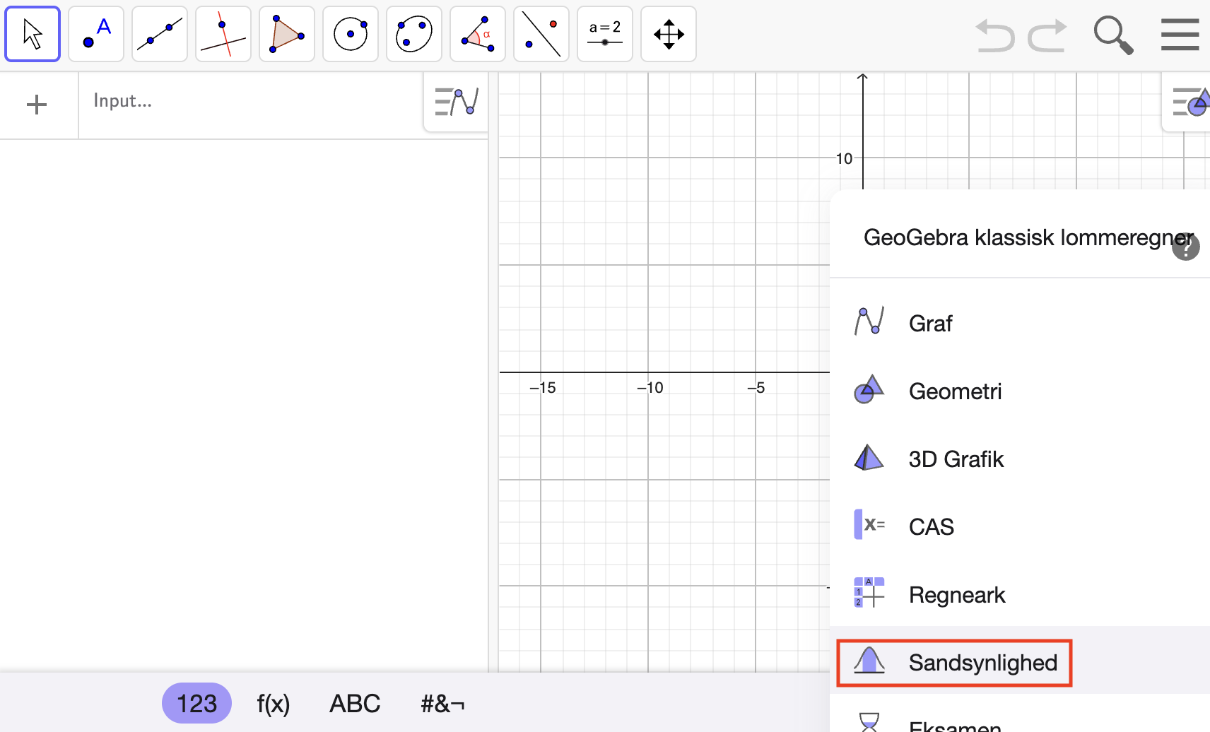
Vi kan regne på kontinuerte fordelinger i GeoGebra på tilsvarende måde, som vi regnede på binomialfordelinger på b-niveau. Vi åbner GeoGebra og åbner sandsynlighedslommeregneren:
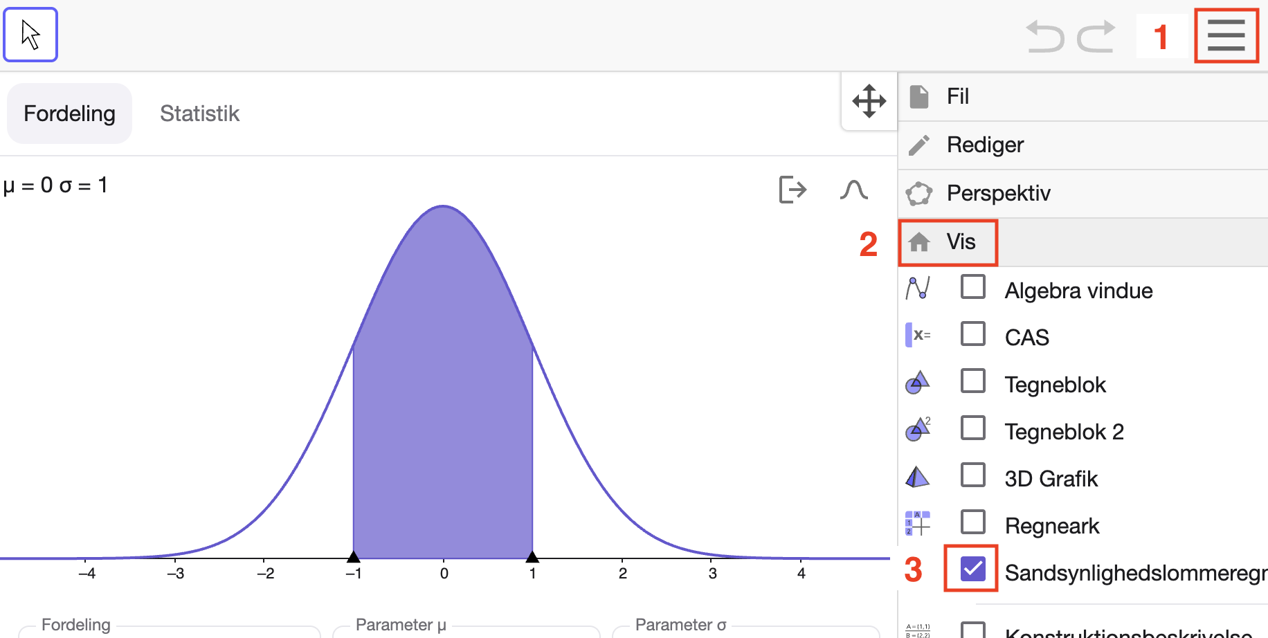
Hvis du missede muligheden, da du åbnede GeoGebra, kan du åbne den som vist her:
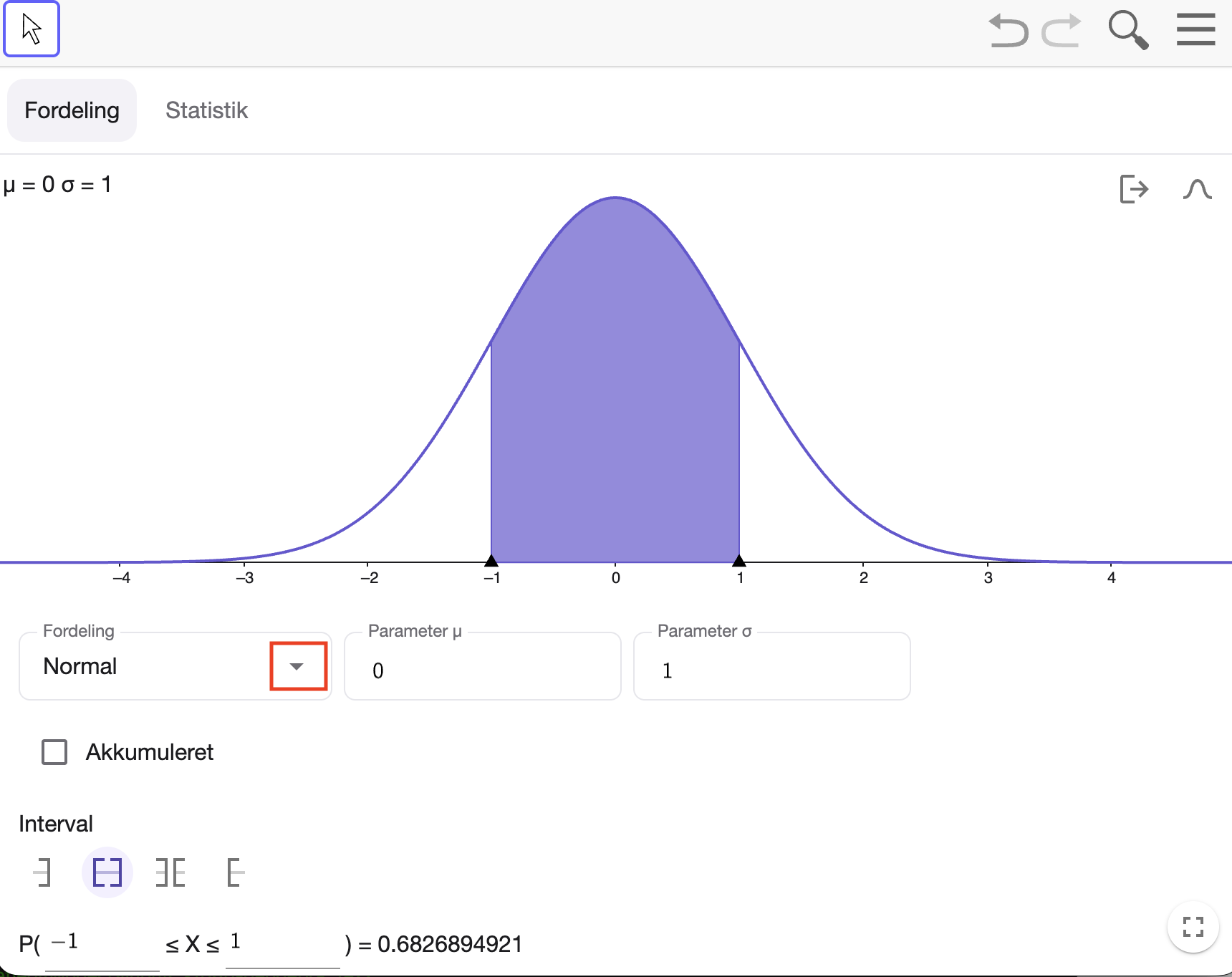
Du kan nu vælge den fordeling, du har brug for:
Prøver man sig lidt frem, er det ikke svært at bruge lommeregneren. Der er dog to ting man skal være opmærksom på, inden man går i gang:
-
1. Man kan kun vælge ”bløde” ulighedstegn (\(\leq \)) og ikke skarpe ulighedstegn (\(<\)). Men det er ikke noget problem, da vi husker, at de giver
samme sandsynligheder for kontinuerte fordelinger.
-
2. Antallet af frihedsgrader betegnes med ”df” i stedet for \(k\) i GeoGebra.
Øvelse 5.8.1
For en normalfordeling \(X\sim N(2,5)\), skal du bestemme følgende sandsynligheder i procent vha. sandsynlighedslommeregneren i GeoGebra:
-
a) \(P(X\leq 3)\)
-
b) \(P(X> 10)\)
-
c) \(P(-5\leq X \leq 5)\)
-
d) Sandsynligheden for at få en værdi, som er mindre end eller lig med \(1\).
-
e) Sandsynligheden for at få en værdi, som er mellem \(3\) og \(6\).
5.8.1
-
a) \(P(X\leq 3)=57{,}93\%\)
-
b) \(P(X> 10)=5{,}48\%\)
-
c) \(P(-5\leq X \leq 5)=64{,}5\%\)
-
d) Sandsynligheden for at få en værdi, som er mindre end \(1\) er \(42{,}07\%\).
-
e) Sandsynligheden for at få en værdi, som er mellem \(3\) og \(6\) er \(20{,}89\%\).
Øvelse 5.8.2
I en intelligenstest måler man en persons intelligenskvotient IQ. I dag er testene konstrueret på en måde, så resultaterne er normalfordelte med en middelværdi på 100 og standardafvigelse på 15. Vi udvælger nu en tilfældig person.
-
a) Hvad er sandsynligheden for, at personens intelligens er under gennemsnittet?
-
b) Hvad er sandsynligheden for, at personen har en IQ på under 80?
-
c) Hvad er sandsynligheden for, at personen har en IQ mellem 80 og 120?
5.8.2
-
a) \(50\%\)
-
b) \(9{,}12\%\)
-
c) \(81{,}76\%\)
Øvelse 5.8.3
En maskine hælder sukker i en pose. Den er indstillet til at hælde \(1050\,\mathrm {g}\) på en pose, men det faktiske indhold er normalfordelt med en middelværdi på \(1050\,\mathrm {g}\) og en standardafvigelse på
\(28\,\mathrm {g}\).
-
a) Bestem sandsynligheden for, at der er under \(1\,\mathrm {kg}\) i en pose.
-
b) Bestem sandsynligheden for, at der er mere end \(1080\,\mathrm {g}\) i en pose.
5.8.3
-
a) \(3{,}71\%\)
-
b) \(14{,}2\%\)
Øvelse 5.8.4
Lad \(X\sim \chi ^2(7)\). Altså \(X\) er \(\chi ^2\)-fordelt med syv frihedsgrader. Bestem:
-
a) \(P(2<X\leq 10)\)
-
b) \(P(X\geq 10)\)
5.8.4
-
a) \(P(2<X\leq 10)=0{,}77\)
-
b) \(P(X\geq 10)=0{,}19\)
Øvelse 5.8.5
Lad \(X\) være \(t\)-fordelt med \(16\) frihedsgrader.
Fraktiler i GeoGebra
Vi har brug for at kunne bestemme fraktiler for både standardnormalfordelingen, \(\chi ^2\)-fordelinger og \(t\)-fordelinger. Vi husker, at en \(p\)-fraktil for en kontinuert fordelt stokastisk variabel \(X\) er et tal \(x_p\), som
opfylder:
\[ P(X\leq x_p) = p \]
Vi bruger følgende betegnelser for \(p\)-fraktiler:
| . |
|---|
| \(z_p\) |
for standardnormalfordelingen |
| \(\chi ^2_p\) |
for chi i anden-fordelinger |
| \(t_p\) |
for t-fordelinger |
-
Eksempel 5.8.1
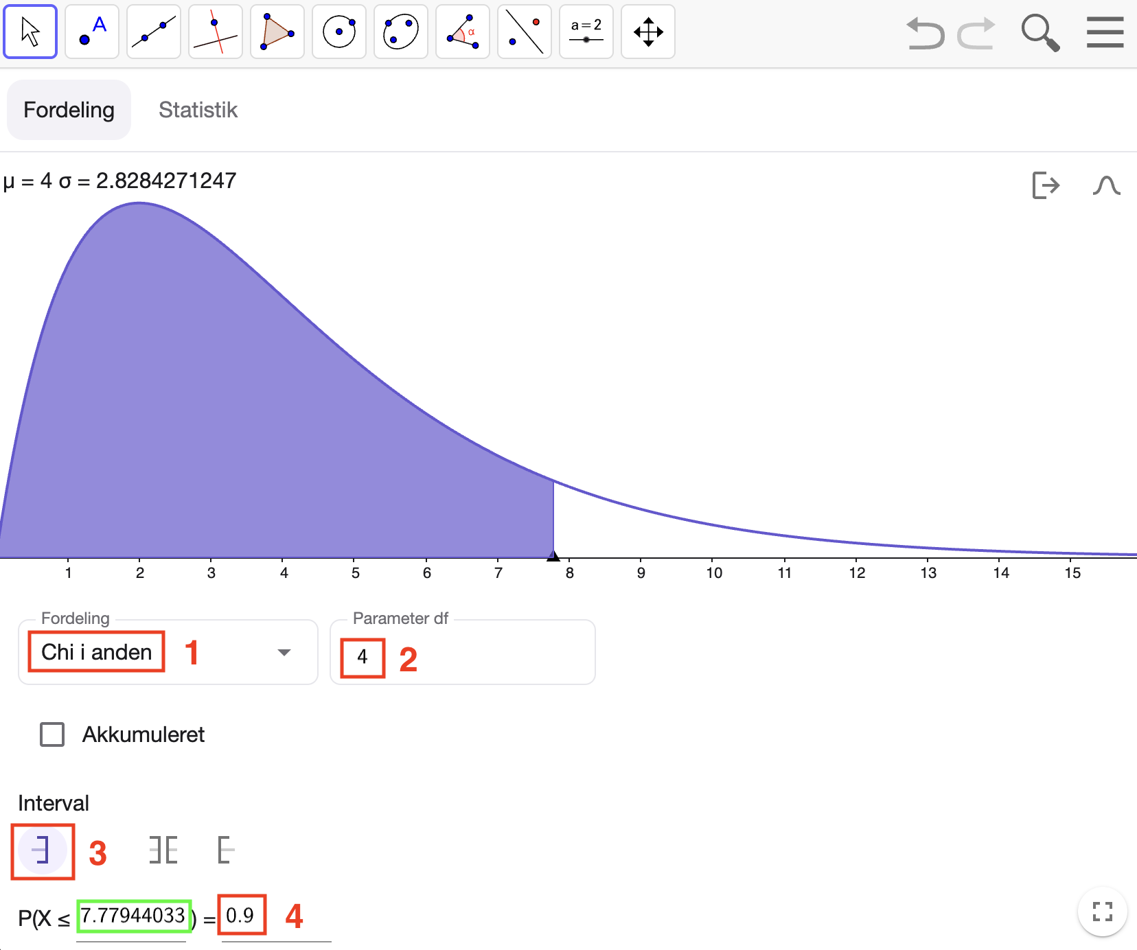
Vi vil bestemme \(\chi ^2_{0{,}975}\) for \(\chi ^2(4)\). Det vil sige, vi skal bestemme \(0{,}975\)-fraktilen i en \(\chi ^2\)-fordeling med fire frihedsgrader. Vi vælger \(\chi
^2\)-fordeling i GeoGebra, taster frihedsgraderne, vælger \(P(X\leq \_\ )\) og taster \(0{,}975\) som sandsynligheden:
Vi ser, at \(\chi ^2_{0{,}975}=7{,}78\).
De kritiske værdier i en \(\chi ^2\)-test er fraktiler i \(\chi ^2\)-fordelinger.
Øvelse 5.8.6
Betragt skemaet:
\[ \begin {array}{| l | l |} \hline k & \chi ^2_{0{,}95}\\ \hline 1 & \\ 2 & \\ 3 & \\ \hline \end {array} \]
5.8.6
-
a) \(\begin {array}{| l | l |} \hline k & \chi ^2_{0{,}95}\\ \hline 1 & 3{,}84\\ 2 & 5{,}99\\ 3 & 7{,}81\\ \hline
\end {array}\)
Når vi bestemmer konfidensintervaller for binomialfordelinger, har vi brug for fraktiler i standardnormalfordelingen. Vi husker, at man først bestemmer signifikansniveauet \(\alpha \) ved:
\[ \alpha = 1 - \text {konfidensniveauet} \]
Derefter kan man regne \(1-\frac {\alpha }{2}\) og så bestemme fraktilerne.
Øvelse 5.8.7
Betragt skemaet:
\(\begin {array}{| l | l |} \hline \alpha & z_{1-\frac {\alpha }{2}} \\ \hline 1\% & \\ 5\% & \\ 10\% & \\ \hline \end {array}\)
5.8.7
-
a) \(\begin {array}{| l | l |} \hline \alpha & z_{1-\frac {\alpha }{2}} \\ \hline 1\% & 2,576 \\ 5\% & 1,960\\ 10\%
& 1,645\\ \hline \end {array}\)
Når vi i næste afsnit skal bestemme konfidensintervaller for middelværdien i en normalfordeling, får vi brug for fraktiler for t-fordelinger. De kan bestemmes i GeoGebra på tilsvarende måde, som fraktiler for \(\chi ^2\)-fordelinger.
Øvelse 5.8.8
Lad \(\alpha =5\%\).